Course
- Notebook Author: Trenton McKinney
- Course: DataCamp: Introduction to Deep Learning in Python
- This notebook was created as a reproducible reference.
- The material is from the course
- The course website uses
tensorflow v2.6.0,scikit-learn v1.0,pandas v1.3.4, andnumpy v1.19.5 - This notebook uses
v2.6.0,v1.3.0,v2.1.4, andv1.26.3respectively, so there are differences in model performance and parameters compared to the course.
- The course website uses
- I completed the exercises with my PC GPU: NVIDIA GeForce RTX 3080 Ti
- If you find the content beneficial, consider a DataCamp Subscription.
- I added a function (
create_dir_save_file) to automatically download and save the required data (data/course_name) and image (Images/course_name) files.
Course Description
Deep learning is the machine learning technique behind the most exciting capabilities in diverse areas like robotics, natural language processing, image recognition, and artificial intelligence, including the famous AlphaGo. In this course, you'll gain hands-on, practical knowledge of how to use deep learning with Keras 2.0, the latest version of a cutting-edge library for deep learning in Python.
Imports
import pandas as pd
from pprint import pprint as pp
from itertools import combinations
from pathlib import Path
import requests
import numpy as np
import sys
import matplotlib.pyplot as plt
import matplotlib.ticker as mtick
from sklearn.metrics import mean_squared_error
from tensorflow.keras import datasets
from tensorflow.keras.layers import Dense
from tensorflow.keras.models import Sequential
from tensorflow.keras import layers
from tensorflow.keras.utils import to_categorical
from tensorflow.keras.optimizers import SGD
from tensorflow.keras.callbacks import EarlyStopping
import tensorflow as tf
tf.config.list_physical_devices('GPU')
[PhysicalDevice(name='/physical_device:GPU:0', device_type='GPU')]
tf testing
# enable the last line to print device placement logging when running `.fit`
# example output: Executing op _EagerConst in device /job:localhost/replica:0/task:0/device:GPU:0
# tf.debugging.set_log_device_placement(True)
# set tf logging levels - 0: Info, 1: Warning, 2: Error, 3: None
# %env TF_CPP_MIN_LOG_LEVEL=3
# Create some tensors
a = tf.constant([[1.0, 2.0, 3.0], [4.0, 5.0, 6.0]])
b = tf.constant([[1.0, 2.0], [3.0, 4.0], [5.0, 6.0]])
c = tf.matmul(a, b)

print(c)
tf.Tensor(
[[22. 28.]
 [49. 64.]], shape=(2, 2), dtype=float32)
Configuration Options
# pd.set_option('max_columns', 200)
# pd.set_option('max_rows', 300)
# pd.set_option('display.expand_frame_repr', True)
# plt.rcParams["patch.force_edgecolor"] = True
Functions
def create_dir_save_file(dir_path: Path, url: str):
    """
    Check if the path exists and create it if it does not.
    Check if the file exists and download it if it does not.
    """
    if not dir_path.parents[0].exists():
        dir_path.parents[0].mkdir(parents=True)
        print(f'Directory Created: {dir_path.parents[0]}')
    else:
        print('Directory Exists')

    if not dir_path.exists():
        r = requests.get(url, allow_redirects=True)
        open(dir_path, 'wb').write(r.content)
        print(f'File Created: {dir_path.name}')
    else:
        print('File Exists')
data_dir = Path('data/2021-04-19_intro_to_deep_learning_in_python')
images_dir = Path('Images/2021-04-19_intro_to_deep_learning_in_python')
Datasets
file_1 = 'https://assets.datacamp.com/production/repositories/654/datasets/8a57adcdb5bfb3e603dad7d3c61682dfe63082b8/hourly_wages.csv'
file_2 = 'https://assets.datacamp.com/production/repositories/654/datasets/24769dae9dc51a77b9baa785d42ea42e3f8f7538/mnist.csv'
file_3 = 'https://assets.datacamp.com/production/repositories/654/datasets/92b75b9bc0c0a8a30999d76f4a1ee786ef072a9c/titanic_all_numeric.csv'
datasets = [file_1, file_2, file_3]
data_paths = list()

for data in datasets:
    file_name = data.split('/')[-1].replace('?raw=true', '')
    data_path = data_dir / file_name
    create_dir_save_file(data_path, data)
    data_paths.append(data_path)
Directory Exists
File Exists
Directory Exists
File Exists
Directory Exists
File Exists
DataFrames
hw: Hourly Wages
hw = pd.read_csv(data_paths[0])
hw.head(2)
| wage_per_hour | union | education_yrs | experience_yrs | age | female | marr | south | manufacturing | construction | |
|---|---|---|---|---|---|---|---|---|---|---|
| 0 | 5.10 | 0 | 8 | 21 | 35 | 1 | 1 | 0 | 1 | 0 |
| 1 | 4.95 | 0 | 9 | 42 | 57 | 1 | 1 | 0 | 1 | 0 |
mnist
mnist = pd.read_csv(data_paths[1], header=None)
mnist.iloc[:2, :6]
| 0 | 1 | 2 | 3 | 4 | 5 | |
|---|---|---|---|---|---|---|
| 0 | 5 | 0 | 0.1 | 0.2 | 0.3 | 0.4 |
| 1 | 4 | 0 | 0.0 | 0.0 | 0.0 | 0.0 |
titanic
titanic = pd.read_csv(data_paths[2])
titanic.head(2)
| survived | pclass | age | sibsp | parch | fare | male | age_was_missing | embarked_from_cherbourg | embarked_from_queenstown | embarked_from_southampton | |
|---|---|---|---|---|---|---|---|---|---|---|---|
| 0 | 0 | 3 | 22.0 | 1 | 0 | 7.2500 | 1 | False | 0 | 0 | 1 |
| 1 | 1 | 1 | 38.0 | 1 | 0 | 71.2833 | 0 | False | 1 | 0 | 0 |
Memory Usage
# These are the usual ipython objects, including this one you are creating
ipython_vars = ['In', 'Out', 'exit', 'quit', 'get_ipython', 'ipython_vars']  # list a variables

# Get a sorted list of the objects and their sizes
sorted([(x, sys.getsizeof(globals().get(x))) for x in dir() if not x.startswith('_') and x not in sys.modules and x not in ipython_vars], key=lambda x: x[1], reverse=True)[:5]
[('mnist', 12566424),
 ('titanic', 72315),
 ('hw', 42864),
 ('Dense', 1064),
 ('EarlyStopping', 1064)]
Basics of deep learning and neural networks
In this chapter, you'll become familiar with the fundamental concepts and terminology used in deep learning, and understand why deep learning techniques are so powerful today. You'll build simple neural networks and generate predictions with them.
Introduction to deep learning
- Imagine you work for a bank
- Imagine you work for a bank, and you need to build a model predicting how many transactions each customer will make next year. You have predictive data or features like:
- Example as seen by linear regression
- each customer’s age,
- bank balance,
- whether they are retired, and so on.
- We'll get to deep learning in a moment, but for comparison, consider how a simple linear regression model works for this problem.
- The linear regression embeds an assumption that the outcome, in this case how many transactions a user makes, is the sum of individual parts.
- It starts by saying, "what is the average?"
- Then it adds the effect of age.
- Then the effect of bank balance. And so on.
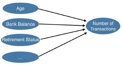
- So the linear regression model isn't identifying the interactions between these parts, and how they affect banking activity.
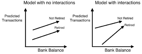
- Say we plot predictions from this model.
- We draw one line with the predictions for retired people, and another with the predictions for those still working.
- We put current bank balance on the horizontal axis, and the vertical axis is the predicted number of transactions.
- The left graph shows predictions from a model with no interactions.
- In that model we simply add up the effect of the retirement status, and current bank balance.
- The lack of interactions is reflected by both lines being parallel.
- That's probably unrealistic, but it's an assumption of the linear regression model.
- The graph on the right shows the predictions from a model that allows interactions, and the lines don't need to be parallel.
- Interactions
- Neural networks are a powerful modeling approach that accounts for interactions like this especially well.
- Deep learning, the focus of this course, is the use of especially powerful neural networks.
- Because deep learning models account for these types of interactions so well, they perform great on most prediction problems you've seen before.
- But their ability to capture extremely complex interactions also allow them to do amazing things with text, images, videos, audio, source code and almost anything else you could imagine doing data science with.
- Course structure
- The first two chapters of this course focus on conceptual knowledge about deep learning.
- This part will be hard, but it will prepare you to debug and tune deep learning models on conventional prediction problems, and it will lay the foundation for progressing towards those new and exciting applications.
- You'll see this pay off in the third and fourth chapter.
- Build and tune deep learning models using keras
- You will write code that looks like this, to build and tune deep learning models using keras, to solve many of the same modeling problems you might have previously solved with scikit-learn.
import numpy as np
from keras.layers import Dense
from keras.models import Sequential
predictors = np.loadtxt('predictors_data.csv', delimiter=',')
n_cols = predictors.shape[1]
model = Sequential()
model.add(Dense(100, activation='relu', input_shape = (n_cols,)))
model.add(Dense(100, activation='relu'))
model.add(Dense(1))
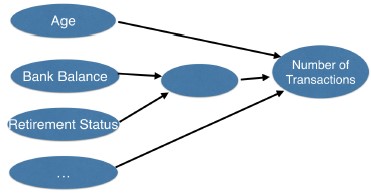
- As a start to how deep learning models capture interactions and achieve these amazing results, we'll modify the diagram you saw a moment ago.
- Deep learning models capture interactions
- Here there is an interaction between retirement status and bank balance.
- Instead of having them separately affect the outcome, we calculate a function of these variables that accounts for their interaction, and use that to predict the outcome.
- Even this graphic oversimplifies reality, where most things interact with each in some way, and real neural network models account for far more interactions.
- So the diagram for a simple neural network looks like this.
- Interactions in neural network
- On the far left, we have something called an input layer. This represents our predictive features like age or income.
- On the far right we have the output layer. The prediction from our model, in this case, the predicted number of transactions.
- All layers that are not the input or output layers are called hidden layers.
- They are called hidden layers because, while the inputs and outputs correspond to visible things that happened in the world, and they can be stored as data, the values in the hidden layer aren't something we have data about, or anything we observe directly from the world.
- Nevertheless, each dot, called a node, in the hidden layer, represents an aggregation of information from our input data, and each node adds to the model's ability to capture interactions.
- So the more nodes we have, the more interactions we can capture.
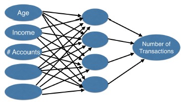
Comparing neural network models to classical regression models
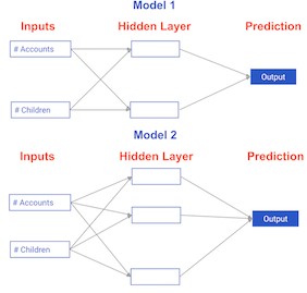
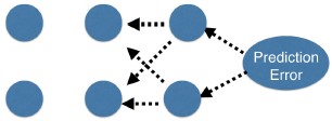
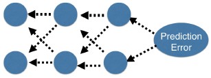
Which of the models in the diagrams has greater ability to account for interactions?
Possible Answers
Model 1.Model 2.
- Model 2 has more nodes in the hidden layer, and therefore, greater ability to capture interactions.
They are both the same.
Forward propagation
- We’ll start by showing how neural networks use data to make predictions. This is called the forward propagation algorithm.
- Bank transactions example
- Let's revisit our example predicting how many transactions a user will make at our bank.
- For simplicity, we'll make predictions based on only the number of children and number of existing accounts.
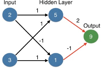
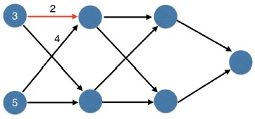
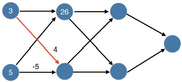
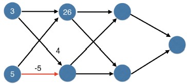
- Forward propagation
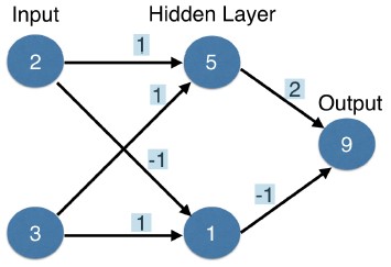
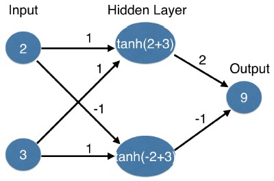
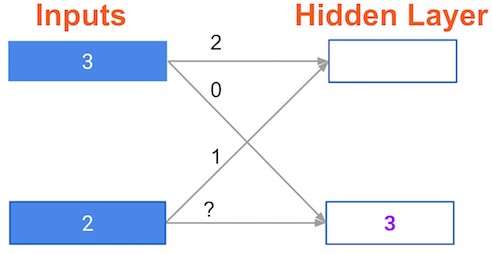
- This graph shows a customer with two children and three accounts.
- The forward-propagation algorithm will pass this information through the network to make a prediction in the output layer.
- Lines connect the inputs to the hidden layer.
- Each line has a weight indicating how strongly that input effects the hidden node that the line ends at.
- These are the first set of weights.
- We have one weight from the top input into the top node of the layer, and one weight from the bottom input to the top node of the hidden layer.
- These weights are the parameters we train or change when we fit a neural network to data, so these weights will be a focus throughout this course.
- To make predictions for the top node of the hidden layer, we take the value of each node in the input layer, multiply it by the weight that ends at that node, and then sum up all the values.
- In this case, we get (2 times 1) plus (3 times 1), which is 5.
- Now do the same to fill in the value of this node on the bottom.
- That is (two times (minus one)) plus (three times one).
- That's one.
- Finally, repeat this process for the next layer, which is the output layer.
- That is (five times two) plus (one times -1).
- That gives an output of 9.
- We predicted nine transactions.
- That's forward-propagation.
- We moved from the inputs on the left, to the hidden layer in the middle, and then from the hidden layers to the output on the right.
- We always use that same multiply then add process.
- If you're familiar with vector algebra or linear algebra, that operation is a dot product.
- If you don't know about dot products, that's fine too.
- That was forward propagation for a single data point.
- In general, we do forward propagation for one data point at a time.
- The value in that last layer is the model's prediction for that data point.
- Forward propagation code
- Let's see the code for this.
- We import Numpy for some of the mathematical operations.
- We've stored the input data as an array. We then have weights into each node in the hidden layer and to the output.
- We store the weights going into each node as an array, and we use a dictionary to store those arrays.
- Let’s start forward propagating. We fill in the top hidden node here, which is called node zero.
- We multiply the inputs by the weights for that node, and then sum both of those terms together.
- Notice that we had two weights for node_0. That matches the two items in the array it is multiplied by, which is the input_data.
- These get converted to a single number by the sum function at the end of the line.
- We then do the same thing for the bottom node of the hidden layer, which is called node 1.
- Now, both node zero and node one have numeric values.
- Forward propagation code
- To simplify multiplication, we put those in an array here.
- If we print out the array, we confirm that those are the values from the hidden layer you saw a moment ago.
- It can also be instructive to verify this by hand with pen and paper.
- To get the output, we multiply the values in the hidden layer by the weights for the output.
- Summing those together gives us 10 minus 1, which is 9.
input_data = np.array([2, 3])
weights = {'node_0': np.array([1, 1]),
'node_1': np.array([-1, 1]),
'output': np.array([2, -1])}
node_0_value = (input_data * weights['node_0']).sum()
node_1_value = (input_data * weights['node_1']).sum()

hidden_layer_values = np.array([node_0_value, node_1_value])
print(hidden_layer_values)

output = (hidden_layer_values * weights['output']).sum()
print(output)
[5 1]
9
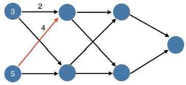
Coding the forward propagation algorithm
In this exercise, you'll write code to do forward propagation (prediction) for your first neural network:
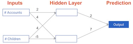
Each data point is a customer. The first input is how many accounts they have, and the second input is how many children they have. The model will predict how many transactions the user makes in the next year. You will use this data throughout the first 2 chapters of this course.
The input data has been pre-loaded as input_data, and the weights are available in a dictionary called weights. The array of weights for the first node in the hidden layer are in weights['node_0'], and the array of weights for the second node in the hidden layer are in weights['node_1'].
The weights feeding into the output node are available in weights['output'].
NumPy will be pre-imported for you as np in all exercises.
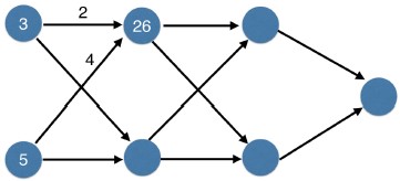
Instructions
Calculate the value in node 0 by multiplying
input_databy its weightsweights['node_0']and computing their sum. This is the 1st node in the hidden layer.Calculate the value in node 1 using
input_dataandweights['node_1']. This is the 2nd node in the hidden layer.Put the hidden layer values into an array. This has been done for you.
Generate the prediction by multiplying
hidden_layer_outputsbyweights['output']and computing their sum.
input_data = np.array([3, 5])
weights = {'node_0': np.array([2, 4]), 'node_1': np.array([ 4, -5]), 'output': np.array([2, 7])}
# Calculate node 0 value: node_0_value
node_0_value = (input_data * weights['node_0']).sum()

# Calculate node 1 value: node_1_value
node_1_value = (input_data * weights['node_1']).sum()

# Put node values into array: hidden_layer_outputs
hidden_layer_outputs = np.array([node_0_value, node_1_value])

# Calculate output: output
output = (hidden_layer_outputs * weights['output']).sum()

# Print output
print(output)
-39
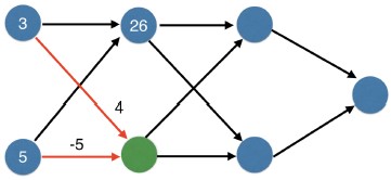
Activation functions
- But creating this multiply-add-process is only half the story for hidden layers. For neural networks to achieve their maximum predictive power, we must apply something called an activation function in the hidden layers.
- Linear vs Nonlinear Functions
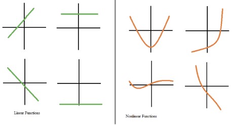
- An activation function allows the model to capture non-linearities.
- Non-linearities, as shown on the right here, capture patterns like how going from no children to one child may impact your banking transactions differently than going from three children to four.
- We have examples of linear functions, straight lines on the left, and non-linear functions on the right.
- If the relationships in the data aren’t straight-line relationships, we will need an activation function that captures non-linearities.
- Activation functions
- An activation function is something applied to the value coming into a node, which then transforms it into the value stored in that node, or the node output.
- Improving our neural network
- Let's go back to the previous diagram. The top hidden node previously had a value of 5.
- For a long time, an s-shaped function called $tanh$ was a popular activation function.
- Activation functions
- If we used the $tanh$ activation function, this node's value would be $tanh(5)$, which is very close to 1.
- Today, the standard in both industry and research applications is something called
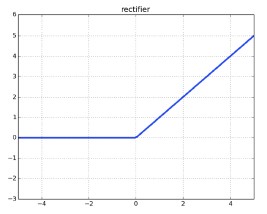
- ReLU (Rectified Linear Activation)
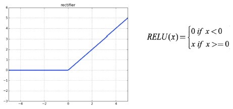
- the ReLU or rectified linear activation function.
- That's depicted here. Though it has two linear pieces, it's surprisingly powerful when composed together through multiple successive hidden layers, which you will see soon.
- The code that incorporates activation functions is shown here.
- Activation functions
- It is the same as the code you saw previously, but we've distinguished the input from the output in each node, which is shown in these lines and then again here.
- And we've applied the $tanh$ function to convert the input to the output.
- That gives us a prediction of 1-point-2 transactions.
input_data = np.array([-1, 2])
weights = {'node_0': np.array([3, 3]), 'node_1': np.array([1, 5]), 'output': np.array([2, -1])}

node_0_input = (input_data * weights['node_0']).sum()
node_0_output = np.tanh(node_0_input)

node_1_input = (input_data * weights['node_1']).sum()
node_1_output = np.tanh(node_1_input)

hidden_layer_outputs = np.array([node_0_output, node_1_output])

output = (hidden_layer_outputs * weights['output']).sum()
output
0.99010953783342
The Rectified Linear Activation Function
As Dan explained to you in the video, an "activation function" is a function applied at each node. It converts the node's input into some output.
The rectified linear activation function (called ReLU) has been shown to lead to very high-performance networks. This function takes a single number as an input, returning 0 if the input is negative, and the input if the input is positive.
Here are some examples:
$relu(3) = 3$
$relu(-3) = 0$
Instructions
- Fill in the definition of the
relu()function: - Use the
max()function to calculate the value for the output ofrelu(). - Apply the
relu()function tonode_0_inputto calculatenode_0_output. - Apply the
relu()function tonode_1_inputto calculatenode_1_output.
def relu
def relu(input_):
    '''Define your relu activation function here'''
    # Calculate the value for the output of the relu function: output
    output = max(0, input_)

    # Return the value just calculated
    return(output)
input_data = np.array([3, 5])
weights = {'node_0': np.array([2, 4]), 'node_1': np.array([ 4, -5]), 'output': np.array([2, 7])}
# Calculate node 0 value: node_0_output
node_0_input = (input_data * weights['node_0']).sum()
node_0_output = relu(node_0_input)

# Calculate node 1 value: node_1_output
node_1_input = (input_data * weights['node_1']).sum()
node_1_output = relu(node_1_input)

# Put node values into array: hidden_layer_outputs
hidden_layer_outputs = np.array([node_0_output, node_1_output])

# Calculate model output (do not apply relu)
model_output = (hidden_layer_outputs * weights['output']).sum()

# Print model output
print(model_output)
52
You predicted 52 transactions. Without this activation function, you would have predicted a negative number! The real power of activation functions will come soon when you start tuning model weights.
Applying the network to many observations/rows of data
You'll now define a function called predict_with_network() which will generate predictions for multiple data observations, which are pre-loaded as input_data. As before, weights are also pre-loaded. In addition, the relu() function you defined in the previous exercise has been pre-loaded.
Instructions
- Define a function called
predict_with_network()that accepts two arguments -input_data_rowandweights- and returns a prediction from the network as the output. - Calculate the input and output values for each node, storing them as:
node_0_input,node_0_output,node_1_input, andnode_1_output.- To calculate the input value of a node, multiply the relevant arrays together and compute their sum.
- To calculate the output value of a node, apply the
relu()function to the input value of the node.
- Calculate the model output by calculating
input_to_final_layerandmodel_outputin the same way you calculated the input and output values for the nodes. - Use a
for loopto iterate overinput_data:- Use your
predict_with_network()to generate predictions for each row of theinput_data-input_data_row. Append each prediction toresults.
- Use your
def predict_with_network1
# Define predict_with_network()
def predict_with_network1(input_data_row, weights):

    # Calculate node 0 value
    node_0_input = (input_data_row * weights['node_0']).sum()
    node_0_output = relu(node_0_input)

    # Calculate node 1 value
    node_1_input = (input_data_row * weights['node_1']).sum()
    node_1_output = relu(node_1_input)

    # Put node values into array: hidden_layer_outputs
    hidden_layer_outputs = np.array([node_0_output, node_1_output])

    # Calculate model output
    input_to_final_layer = (hidden_layer_outputs * weights['output']).sum()
    model_output = relu(input_to_final_layer)

    # Return model output
    return(model_output)
input_data = [np.array([3, 5]), np.array([ 1, -1]), np.array([0, 0]), np.array([8, 4])]
weights = {'node_0': np.array([2, 4]), 'node_1': np.array([ 4, -5]), 'output': np.array([2, 7])}
# Create empty list to store prediction results
results = []
for input_data_row in input_data:
    # Append prediction to results
    results.append(predict_with_network1(input_data_row, weights))

# Print results
print(results)
[52, 63, 0, 148]
Deeper networks
- The difference between modern deep learning and the historical neural networks that didn't deliver these amazing results, is the use of models with not just one hidden layer, but with many successive hidden layers.
- We forward propagate through these successive layers in a similar way to what you saw for a single hidden layer.
- Multiple hidden layers
- Here is a network with two hidden layers. We first fill in the values for hidden layer one as a function of the inputs.
- Then apply the activation function to fill in the values in these nodes.
- Then use values from the first hidden layer to fill in the second hidden layer.
- Then we make a prediction based on the outputs of hidden layer two.
- In practice, it's becoming common to have neural networks that have many, many layers; five layers, ten layers.
- A few years ago 15 layers was state of the art but this can scale quite naturally to even a thousand layers.
- You use the same forward propagation process, but you apply that iterative process more times.
- Let's walk through the first steps of that.
- Assume all layers here use the ReLU activation function.
- We'll start by filling in the top node of the first hidden layer.
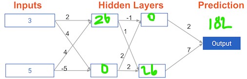
- That will use these two weights.
- The top weights contributes 3 times 2, or 6.
- The bottom weight contributes 20.
- The ReLU activation function on a positive number just returns that number.
- So we get 26.
- Now let's do the bottom node of that first hidden layer.
- We use these two nodes.
- Using the same process, we get 4 times 3, or 12 from this weight.
- And -25 from the bottom weight.
- So the input to this node is 12 minus 25.
- Recall that, when we apply ReLU to a negative number, we get 0.
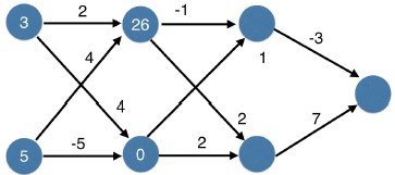
- So this node is 0.
- We've shown the values for the subsequent layers here.
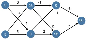
- Pause this video, and verify you can calculate the same values at each node.
- At this point, you understand the mechanics for how neural networks make predictions.
- Let's close this chapter with an interesting and important fact about these deep networks.
- Representation learning
- That is, they internally build up representations of the patterns in the data that are useful for making predictions.
- And they find increasingly complex patterns as we go through successive hidden layers of the network.
- In this way, neural networks partially replace the need for feature engineering, or manually creating better predictive features.
- Deep learning is also sometimes called representation learning, because subsequent layers build increasingly sophisticated representations of the raw data, until we get to a stage where we can make predictions.
- This is easiest to understand from an application to images, which you will see later in this course.
- Even if you haven't worked with images, you may find it useful to think through this example heuristically.
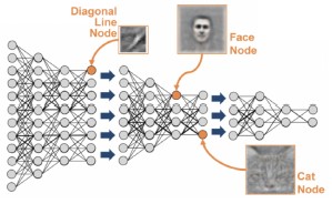
- Representation learning
- When a neural network tries to classify an image, the first hidden layers build up patterns or interactions that are conceptually simple.
- A simple interaction would look at groups of nearby pixels and find patterns like diagonal lines, horizontal lines, vertical lines, blurry areas, etc.
- Once the network has identified where there are diagonal lines and horizontal lines and vertical lines, subsequent layers combine that information to find larger patterns, like big squares.
- A later layer might put together the location of squares and other geometric shapes to identify a checkerboard pattern, a face, a car, or whatever is in the image.
- The cool thing about deep learning is that the modeler doesn't need to specify those interactions.
- Deep learning
- We never tell the model to look for diagonal lines.
- Instead, when you train the model, which you'll learn to do in the next chapter, the network gets weights that find the relevant patterns to make better predictions.
- Working with images may still seem abstract, but this idea of finding increasingly complex or abstract patterns is a recurring theme when people talk about deep learning, and it will feel more concrete as you work with these networks more.
Forward propagation in a deeper network
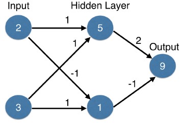
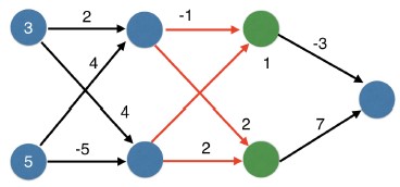
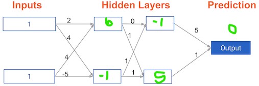
You now have a model with 2 hidden layers. The values for an input data point are shown inside the input nodes. The weights are shown on the edges/lines. What prediction would this model make on this data point?
Assume the activation function at each node is the identity function. That is, each node's output will be the same as its input. So the value of the bottom node in the first hidden layer is -1, and not 0, as it would be if the ReLU activation function was used.
Possible Answers
0.
7.9.
Multi-layer neural networks
In this exercise, you'll write code to do forward propagation for a neural network with 2 hidden layers. Each hidden layer has two nodes. The input data has been preloaded as input_data. The nodes in the first hidden layer are called node_0_0 and node_0_1. Their weights are pre-loaded as weights['node_0_0'] and weights['node_0_1'] respectively.
The nodes in the second hidden layer are called node_1_0 and node_1_1. Their weights are pre-loaded as weights['node_1_0'] and weights['node_1_1'] respectively.
We then create a model output from the hidden nodes using weights pre-loaded as weights['output'].
Instructions
Calculate
node_0_0_inputusing its weightsweights['node_0_0']and the giveninput_data. Then apply therelu()function to getnode_0_0_output.Do the same as above for
node_0_1_inputto getnode_0_1_output.Calculate
node_1_0_inputusing its weightsweights['node_1_0']and the outputs from the first hidden layer -hidden_0_outputs. Then apply therelu()function to getnode_1_0_output.Do the same as above for
node_1_1_inputto getnode_1_1_output.Calculate
model_outputusing its weightsweights['output']and the outputs from the second hidden layerhidden_1_outputsarray. Do not apply therelu()function to this output.
def predict_with_network2
def predict_with_network2(input_data, weights):
    # Calculate node 0 in the first hidden layer
    node_0_0_input = (input_data * weights['node_0_0']).sum()
    node_0_0_output = relu(node_0_0_input)

    # Calculate node 1 in the first hidden layer
    node_0_1_input = (input_data * weights['node_0_1']).sum()
    node_0_1_output = relu(node_0_1_input)

    # Put node values into array: hidden_0_outputs
    hidden_0_outputs = np.array([node_0_0_output, node_0_1_output])

    # Calculate node 0 in the second hidden layer
    node_1_0_input = (hidden_0_outputs * weights['node_1_0']).sum()
    node_1_0_output = relu(node_1_0_input)

    # Calculate node 1 in the second hidden layer
    node_1_1_input = (hidden_0_outputs * weights['node_1_1']).sum()
    node_1_1_output = relu(node_1_1_input)

    # Put node values into array: hidden_1_outputs
    hidden_1_outputs = np.array([node_1_0_output, node_1_1_output])

    # Calculate model output: model_output
    model_output = relu((hidden_1_outputs * weights['output']).sum())

    # Return model_output
    return(model_output)
input_data = np.array([3, 5])
weights = {'node_0_0': np.array([2, 4]),
           'node_0_1': np.array([ 4, -5]),
           'node_1_0': np.array([-1,  2]),
           'node_1_1': np.array([1, 2]),
           'output': np.array([2, 7])}
output = predict_with_network2(input_data, weights)
print(output)
182
Representations are learned
How are the weights that determine the features/interactions in Neural Networks created?
Possible Answers
A user chooses them when creating the model.- The model training process sets them to optimize predictive accuracy.
The weights are random numbers.
Levels of representation
Which layers of a model capture more complex or "higher level" interactions?
Possible Answers
The first layers capture the most complex interactions.- The last layers capture the most complex interactions.
All layers capture interactions of similar complexity.
Optimizing a neural network with backward propagation
Learn how to optimize the predictions generated by your neural networks. You'll use a method called backward propagation, which is one of the most important techniques in deep learning. Understanding how it works will give you a strong foundation to build on in the second half of the course.
The need for optimization
- You've seen the forward-propagation algorithm that neural networks use to make predictions.
- However, the mere fact that a model has the structure of a neural network does not guarantee that it will make good predictions.
- A baseline neural network
- To see the importance of model weights, we'll go back to a network you saw in the previous chapter.
- We'll use a simple example for the sake of explanation.
- For the moment, we won't use an activation function in this example, or if you prefer, you might think of an activation function that returns the input, sometimes called the identity function.
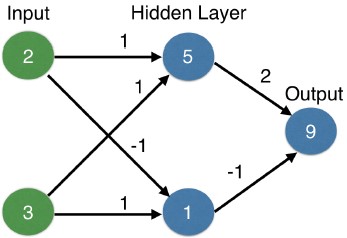
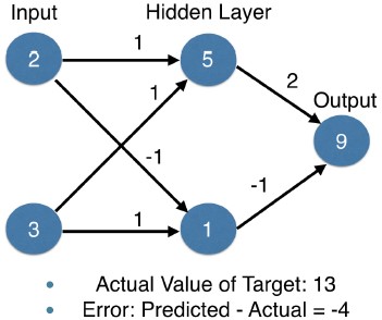
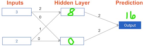
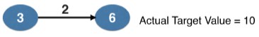
- We have values of 2 and 3 for the inputs, and the true value of the target is 13.
- So, the closer our prediction is to 13, the more accurate this model is for this data point.
- We use forward propagation to fill in the values of hidden layer.
- That gives us hidden node values of 5 and 1.
- Continuing forward propagation, we use those hidden node values to make a prediction of 9.
- Since the true target value is 13, our error is 13 minus 9, which is 4.
- Changing any weight will change our prediction.
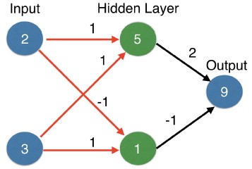
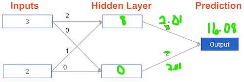
- Let's see what happens if we change the two weights from the hidden layer to the output.
- In this case, we make the top weight 3 and the bottom weight -2.
- Now forward propagation gives us a prediction of 13.
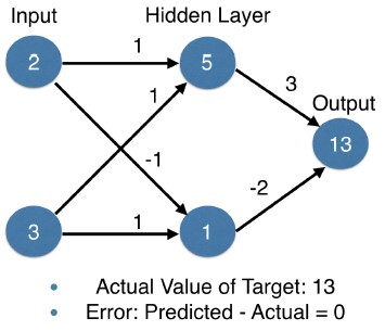
- That is exactly the value we wanted to predict.
- So, this change in weights improved the model for this data point.
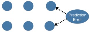
- Predictions with multiple points
- Making accurate predictions gets harder with multiple points.
- First of all, at any set of weights, we have many values of the error, corresponding to the many points we make predictions for.
- Loss function
- We use something called a loss function to aggregate all the errors into a single measure of the model's predictive performance.
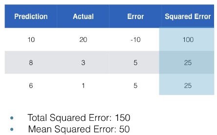
- Squared error loss function
- For example, a common loss function for regression tasks is mean-squared error.
- You square each error, and take the average of that as a measure of model quality.
- The loss function aggregates all of the errors into a single score.
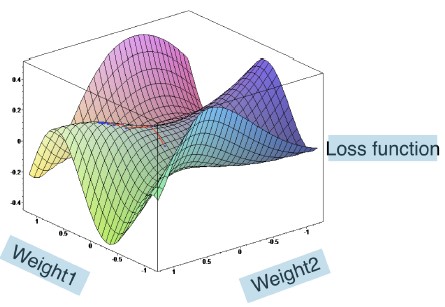
- Loss function
- For an illustration, consider a model with only two weights, we could plot the model's performance for each set of weights like this.
- The values of the weights are plotted on the x and y axis, and the loss function is on the vertical or z axis.
- Lower values mean a better model, so our goal is to find the weights giving the lowest value for the loss function.
- We do this with an algorithm called gradient descent.
- An analogy may be helpful.
- Gradient descent
- Imagine you are in a pitch dark field, and you want to find the lowest point.
- You might feel the ground to see how it slopes, and take a small step downhill.
- This gives an improvement, but not necessarily the lowest point yet.
- So you repeat this process until it is uphill in every direction.
- This is roughly how gradient descent works.
- Gradient descent steps
- The steps are: Start at a random point, until you are somewhere flat, find the slope, and take a step downhill.
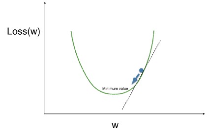
- Optimizing a model with a single weight
- Let's look at optimizing a model with a single weight, and then we'll scale up to optimizing multiple weights.
- We have a curve showing the loss function on the vertical axis, at different values of the weight, which is on the horizontal axis.
- We are looking for the low point on this curve, because that means our model is as accurate as possible.
- We have drawn this tangent line to the curve at our current point.
- The slope of that tangent line captures the slope of the loss function at the our current weight.
- That slope corresponds to something called the derivative from calculus. We use this slope to decide what direction we step.
- In this case, the slope is positive.
- So if we want to go downhill, we go in the direction opposite the slope, towards lower numbers.
- If we repeatedly take small steps opposite the slope, recalculating the slope each time, we will eventually get to the minimum value.
Calculating model errors
For the exercises in this chapter, you'll continue working with the network to predict transactions for a bank.
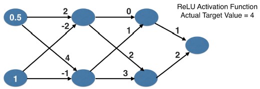
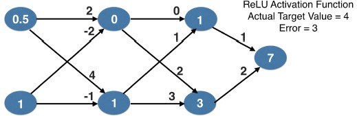
What is the error (predicted - actual) for the following network using the ReLU activation function when the input data is [3, 2] and the actual value of the target (what you are trying to predict) is 5? It may be helpful to get out a pen and piece of paper to calculate these values.
Possible Answers
5.6.11.
- The network generates a prediction of
16, which results in an error of11.
- The network generates a prediction of
16.
Understanding how weights change model accuracy
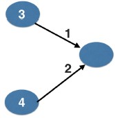
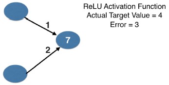
Imagine you have to make a prediction for a single data point. The actual value of the target is 7. The weight going from node_0 to the output is 2, as shown below. If you increased it slightly, changing it to 2.01, would the predictions become more accurate, less accurate, or stay the same?
Possible Answers
More accurate.Less accurate.
- Increasing the weight to
2.01would increase the resulting error from9to9.08, making the predictions less accurate.
- Increasing the weight to
Stay the same.
Coding how weight changes affect accuracy
Now you'll get to change weights in a real network and see how they affect model accuracy!
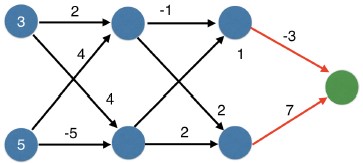
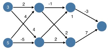
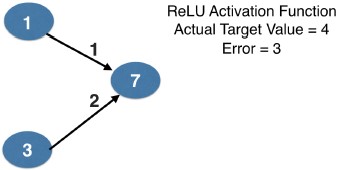
Have a look at the following neural network:
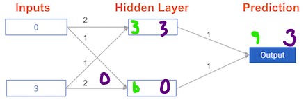
Its weights have been pre-loaded as weights_0. Your task in this exercise is to update a single weight in weights_0 to create weights_1, which gives a perfect prediction (in which the predicted value is equal to target_actual: 3).
Use a pen and paper if necessary to experiment with different combinations. You'll use the predict_with_network() function, which takes an array of data as the first argument, and weights as the second argument.
Instructions
Create a dictionary of weights called
weights_1where you have changed 1 weight fromweights_0(You only need to make 1 edit toweights_0to generate the perfect prediction).Obtain predictions with the new weights using the
predict_with_network()function withinput_dataandweights_1.Calculate the error for the new weights by subtracting
target_actualfrommodel_output_1.
# The data point you will make a prediction for
input_data = np.array([0, 3])

# Sample weights
weights_0 = {'node_0': [2, 1],
             'node_1': [1, 2],
             'output': [1, 1]
            }

# The actual target value, used to calculate the error
target_actual = 3

# Make prediction using original weights
model_output_0 = predict_with_network1(input_data, weights_0)

# Calculate error: error_0
error_0 = model_output_0 - target_actual
error_0
6
# Create weights that cause the network to make perfect prediction (3): weights_1
weights_1 = {'node_0': [2, 1],
             'node_1': [1, 0],
             'output': [1, 1]
            }

# Make prediction using new weights: model_output_1
model_output_1 = predict_with_network1(input_data, weights_1)

# Calculate error: error_1
error_1 = model_output_1 - target_actual

# Print error_1
error_1
0
Scaling up to multiple data points
You've seen how different weights will have different accuracies on a single prediction. But usually, you'll want to measure model accuracy on many points. You'll now write code to compare model accuracies for two different sets of weights, which have been stored as weights_0 and weights_1.
input_data is a list of arrays. Each item in that list contains the data to make a single prediction. target_actuals is a list of numbers. Each item in that list is the actual value we are trying to predict.
In this exercise, you'll use the mean_squared_error() function from sklearn.metrics. It takes the true values and the predicted values as arguments.
You'll also use the preloaded predict_with_network() function, which takes an array of data as the first argument, and weights as the second argument.
Instructions
- Import
mean_squared_error fromsklearn.metrics. - Using a
for loopto iterate over each row ofinput_data:- Make predictions for each row with
weights_0using thepredict_with_network()function and append it tomodel_output_0. - Do the same for
weights_1, appending the predictions tomodel_output_1.
- Make predictions for each row with
- Calculate the mean squared error of
model_output_0and thenmodel_output_1using themean_squared_error()function. The first argument should be the actual values (target_actuals), and the second argument should be the predicted values (model_output_0ormodel_output_1).
weights_0 = {'node_0': np.array([2, 1]), 'node_1': np.array([1, 2]), 'output': np.array([1, 1])}
weights_1 = {'node_0': np.array([2, 1]), 'node_1': np.array([1. , 1.5]), 'output': np.array([1. , 1.5])}
input_data = [np.array([0, 3]), np.array([1, 2]), np.array([-1, -2]), np.array([4, 0])]
target_actuals = [1, 3, 5, 7]
# from sklearn.metrics import mean_squared_error

# Create model_output_0
model_output_0 = []
# Create model_output_1
model_output_1 = []

# Loop over input_data
for row in input_data:
    # Append prediction to model_output_0
    model_output_0.append(predict_with_network1(row, weights_0))

    # Append prediction to model_output_1
    model_output_1.append(predict_with_network1(row, weights_1))

# Calculate the mean squared error for model_output_0: mse_0
mse_0 = mean_squared_error(target_actuals, model_output_0)

# Calculate the mean squared error for model_output_1: mse_1
mse_1 = mean_squared_error(target_actuals, model_output_1)

# Print mse_0 and mse_1
print(f"Mean squared error with weights_0: %{round(mse_0, 2)}")
print(f"Mean squared error with weights_1: %{round(mse_1, 2)}")
Mean squared error with weights_0: %37.5
Mean squared error with weights_1: %49.89
model_output_1 has a higher mean squared error.
Gradient descent
- With gradient descent, you repeatedly repeatedly found a slope capturing how your loss function changes as a weight changes.
- You then made a small change to the weight to get to a lower point, and you repeated this until you couldn't go downhill any more.
- If the slope is positive:
- going opposite the slope means moving to lower numbers.
- Subtracting the slope from the current value achieves this.
- Too big a step might lead us far astray.
- So, instead of directly subtracting the slope, we multiply the slope by a small number, called the learning rate, and we change the weight by the product of that multiplication.
- Learning rate are frequently around point-01.
- This ensures we take small steps, so we reliably move towards the optimal weights.
- But how do we find the relevant slope for each weight we need to update? Working this out for yourself involves calculus, especially the application of the chain rule.
- Don't worry if you don't remember or don't know the underlying calculus.
- We'll explain some basic concepts here, and Keras and TensorFlow do the calculus for us.
- Gradient Descent animation: 1. Simple linear Regression
- Slope calculation example
- Here is a first example to calculate a slope for a weight, and in this example we will look at a single data point.
- Weights feed from one node into another, and you always get the slope you need by multiplying three things.
- First, the slope of the loss function with respect to the value at the node we feed into.
- Second, the value of the node that feeds into our weight.
- Third, the slope of the activation function with respect to the value we feed into.
- Let's start with the slope of the loss function with respect to the value of the node our weight feeds into.
- In this case, that node is the model's prediction.
- If you work through some calculus, you will find that the slope of the mean-squared loss function with respect to the prediction is $2 * (predicted value - actual value)$.
- Which is $2 * error$.
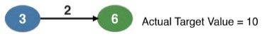
- Here, the prediction from forward propagation was $6$.
- The actual target value is $10$, so the error is $6 - 10$, which is $-4$.
- The second thing we multiply is the value at the node we are feeding from. Here, that is 3.
- Finally, the slope of the activation function at the value we feed into.
- Since we don't have an activation function here, we can leave that out.
- So our final result for the slope of the loss if we graphed it against this weight is $2 * -4 * 3$, or $-24$.
- We would now improve this weight by subtracting the learning rate times that slope, $-24$.
- If the learning rate were $0.01$, we would update this weight to be $2.24$.
- That gives us a better model.
- And it would continue improving if we repeated this process.
- For multiple weights feeding to the output, we repeat this calculation separately for each weight.
- Then we update both weights simultaneously using their respective derivatives.
- Network with two inputs affecting prediction
- Here is a network with two weights going directly to an output, and again with no activation function.
- Let's see the code to calculate slopes and update the weights.
- First, we set up the weights, input data, and a target value to predict.
- Code to calculate slopes and update weights
- Here is the slope calculation.
- We uses numpy broadcasting, which multiplies an array by a number so that each entry in the array is multiplied by that number.
- We multiply the two times the error times the array with the input nodes.
- This gives us an array that used the 1st node value for the first calculated slope, and the second node value for the 2nd calculated slope.
- This is exactly what we wanted. Incidentally, the mathematical term for this array of slopes is a "gradient", and this is where the name gradient descent comes from.
- We update the weights by some small step in that direction, where the step size is partially determined by the learning rate.
- And the new error is $2.5$, which is an improvement over the old error, which was $5$.
- Repeating that process from the new values would give further improvements.
weights = np.array([1, 2])
input_data = np.array([3, 4])
target = 6
learning_rate = 0.01
preds = (weights * input_data).sum()
error = preds - target
error
5
gradient = 2 * input_data * error
gradient
array([30, 40])
weights_updated = weights - learning_rate * gradient
preds_updated = (weights_updated * input_data).sum()
error_updated = preds_updated - target
error_updated
2.5
Calculating slopes
You're now going to practice calculating slopes. When plotting the mean-squared error loss function against predictions, the slope is:
- $2 * x * (xb-y)$
- $2 * input\_data * error$.
Note that $x$ and $b$ may have multiple numbers ($x$ is a vector for each data point, and $b$ is a vector). In this case, the output will also be a vector, which is exactly what you want.
You're ready to write the code to calculate this slope while using a single data point. You'll use pre-defined weights called weights as well as data for a single point called input_data. The actual value of the target you want to predict is stored in target.
Instructions
- Calculate the predictions,
preds, by multiplyingweightsby theinput_dataand computing their sum. - Calculate the error, which is
predsminustarget. Notice that this error corresponds to $xb-y$ in the gradient expression. - Calculate the slope of the loss function with respect to the prediction. To do this, you need to take the product of
input_dataanderrorand multiply that by $2$.
def get_slope
def get_slope(input_data, target, weights):
    # Calculate the predictions: preds
    preds = (weights * input_data).sum()

    # Calculate the error: error
    error = preds - target

    # Calculate the slope: slope
    slope = 2 * input_data * error

    return slope
weights = np.array([0, 2, 1])
input_data = np.array([1, 2, 3])
target = 0
get_slope(input_data, target, weights)
array([14, 28, 42])
Improving model weights
You've just calculated the slopes you need. Now it's time to use those slopes to improve your model. If you add the slopes to your weights, you will move in the right direction. However, it's possible to move too far in that direction. So you will want to take a small step in that direction first, using a lower learning rate, and verify that the model is improving.
The weights have been pre-loaded as weights, the actual value of the target as target, and the input data as input_data. The predictions from the initial weights are stored as preds.
Instructions
- Set the learning rate to be $0.01$ and calculate the error from the original predictions. This has been done for you.
- Calculate the updated weights by subtracting the product of
learning_rateandslopefromweights. - Calculate the updated predictions by multiplying
weights_updatedwithinput_dataand computing their sum. - Calculate the error for the new predictions. Store the result as
error_updated.
# Set the learning rate: learning_rate
learning_rate = 0.01
# Calculate the predictions: preds
preds = (weights * input_data).sum()

# Calculate the error: error
error = preds - target

# Calculate the slope: slope
slope = 2 * input_data * error
# Update the weights: weights_updated
weights_updated = weights - learning_rate * slope

# Get updated predictions: preds_updated
preds_updated = (weights_updated * input_data).sum()

# Calculate updated error: error_updated
error_updated = preds_updated - target

# Print the original error
print(error)

# Print the updated error
print(error_updated)
7
5.04
Making multiple updates to weights
You're now going to make multiple updates so you can dramatically improve your model weights, and see how the predictions improve with each update.
To keep your code clean, there is a pre-loaded get_slope() function that takes input_data, target, and weights as arguments. There is also a get_mse() function that takes the same arguments. The input_data, target, and weights have been pre-loaded.
This network does not have any hidden layers, and it goes directly from the input (with 3 nodes) to an output node. Note that weights is a single array.
We have also pre-loaded matplotlib.pyplot, and the error history will be plotted after you have done your gradient descent steps.
Instructions
- Using a
for loopto iteratively update weights: - Calculate the slope using the
get_slope()function. - Update the weights using a learning rate of $0.01$.
- Calculate the mean squared error (
mse) with the updated weights using theget_mse()function. - Append
msetomse_hist. - What trend do you notice?
def get_mse
def get_mse(input_data, target, weights):

    preds = (weights * input_data).sum()
    mse = mean_squared_error([target], [preds])
    return mse
weights = np.array([0, 2, 1])
input_data = np.array([1, 2, 3])
target = 0

n_updates = 20
mse_hist = []

# Iterate over the number of updates
for i in range(n_updates):
    # Calculate the slope: slope
    slope = get_slope(input_data, target, weights)

    # Update the weights: weights
    weights = weights - 0.01 * slope

    # Calculate mse with new weights: mse
    mse = get_mse(input_data, target, weights)

    # Append the mse to mse_hist
    mse_hist.append(mse)
# Plot the mse history
plt.plot(mse_hist)
plt.xlabel('Iterations')
plt.ylabel('Mean Squared Error')
plt.gca().yaxis.set_major_formatter(mtick.PercentFormatter())
plt.show()

As you can see, the mean squared error decreases as the number of iterations go up.
Backpropagation
- You've used gradient descent to optimize weights in a simple model.
- Now we'll add a technique called "back propagation" to calculate the slopes you need to optimize more complex deep learning models.
- Just as forward propagation sends input data through the hidden layers and into the output layer, back propagation takes the error from the output layer and propagates it backward through the hidden layers, towards the input layer.
- It calculates the necessary slopes sequentially from the weights closest to the prediction, through the hidden layers, eventually back to the weights coming from the inputs.
- We then use these slopes to update our weights as you've seen.
- Back propagation is tricky, so you should focus on the general structure of the algorithm, rather than trying to memorize every mathematical detail.
- Backpropagation process
- In the big picture, we are trying to estimate the slope of the loss function with respect to each weight in our network.
- You've already seen that we use prediction errors to calculate some of those slopes.
- So we always do forward propagation to make a prediction and calculate an error before we do back propagation.
- Here are the results of forward propagation. Node values are in white and weights are in black.
- We need to be at this step before we can start back-propagation.
- Notice, we are using the "relu" activation function.
- So any node whose input is negative takes a value of 0, and that happens in the top node of the first hidden layer.
- For back-propagation, we go back one layer at a time, and each time we go back a layer, we'll use a formula for slopes that you saw in the last video.
- Every weight feeds from some input node into some output node.
- The three things we multiply to get the slope for that weight are
- the value at the weights input node
- the slope from plotting the loss function against that weight's output node
- the slope of the activation function at the weight's output.
- We know the value at the node feeding into this weight.
- Either it is in an input layer, in which case we have it from the data. Or that node is in a hidden layer, in which case we calculated its value when we did forward propagation.
- The second item on this list is the slope of the loss function with respect to the output node.
- We do backward propagation from the right side of our diagram to the left.
- So we already calculated that slope by the time we to plug it into the current calculation.
- Finally we need the slope of the activation function at the node it feeds into.
- ReLU Activation Function
- You can see from this diagram that, for the ReLU function, the slope is 0 if the input into a node is negative.
- If the input into the node is positive, the output is the same as the input.
- So the slope would be 1.
- Backpropagation process
- So far, we have focused on calculating slopes of the loss function with respect to weights.
- We also keep track of the slopes of the loss function with respect to node values, because we use those slopes in our calculations of slopes at weights.
- The slope of the loss function with respect to any node value is the sum of the slopes for every weight coming into that node.
The relationship between forward and backward propagation
If you have gone through 4 iterations of calculating slopes (using backward propagation) and then updated weights, how many times must you have done forward propagation?
Possible Answers
0.1.- 4.
- Each time you generate predictions using forward propagation, you update the weights using backward propagation.
8.
Thinking about backward propagation
If your predictions were all exactly right, and your errors were all exactly 0, the slope of the loss function with respect to your predictions would also be 0. In that circumstance, which of the following statements would be correct?
Possible Answers
- The updates to all weights in the network would also be 0.
- In this situation, the updates to all weights in the network would indeed also be 0
The updates to all weights in the network would be dependent on the activation functions.The updates to all weights in the network would be proportional to values from the input data.
Backpropagation in practice
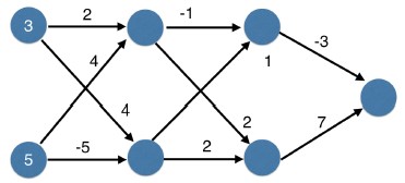
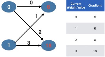
- Let's see this back propagation in a deeper network.
- Backpropagation
- Start at the last set of weights.
- Those are currently 1 and 2.
- We multiply 3 things.
- The node values feeding into these weights are 1 and 3.
- The relevant slope for the output node is 2 times the error.
- That's 6. And the slope of the activation function is 1, since the output node is positive.
- So, we have a slope for the top weight of 6, and a slope for the bottom weight of 18.
- Those slopes we just calculated feed into the formula associated with weights further back in the network.
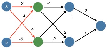
- Let's do that calculation one layer back now. We've hidden the earlier and later layers, since we don't need them to calculate the slopes for this layer of the network.
- This graph uses white to denotes node values, black to denote weight values, and the red shows the calculated slopes of the loss function with respect to that node, which we just finished calculating.
- This is all the information we need to calculate the slopes of the loss function with respect to the weights in this diagram.
- Calculating slopes associated with any weight
- Recall, the three things we multiply to get slopes associated with any weight:
- value at the node feeding into the weight
- the slope of the activation function for the node being fed into (that slope is 1 in all cases here)
- the slope of the loss function with respect to the output node
- Recall, the three things we multiply to get slopes associated with any weight:
- Backpropagation
- Let's start with the slopes related to the weights going into the top node.
- For the top weight going into the top node, we multiply 0 for the input node's value, which is in white.
- Times 6 for the output node's slope, which is in red.
- Times the derivative of the ReLU activation function.
- That output node has a positive value for the input, so the ReLU activation has a slope of 1 (e.g. 0 times 6 times 1 is 0.)
- For the other weight going into this node, we have 1 times 6 times the slope of the ReLU activation function at the output node's value.
- The slope of the activation function is still 1.
- So, we have 1 times 6 times 1, which is 6.
- Here we also show slopes associated with the other two weights.
- We would multiply them all by a learning rate, and use the results to update the weights in gradient descent.
- Pause the video and make sure you understand how these last two weights were calculated.
- You are through the hardest concepts in this course, which are gradient descent and back-propagation.
- Backpropagation: Recap
- As a recap, we start at some random set of weights.
- We then go through the following iterative process
- Use forward propagation to make a prediction.
- Use backward propagation to calculate the slope of the loss function with respect to each weight.
- Multiply that slope by the learning rate, and subtract that from the current weights.
- Keep going with that cycle until we get to a flat part.
- Stochastic gradient descent
- For computational efficiency, it is common to calculate slopes on only a subset of the data, called a batch, for each update of the weights.
- You then use a different batch of data to calculate the next update.
- Once we have used all our data, we start over again at the beginning of the data.
- Each time through the full training data is called an epoch.
- So if we're going through our data for the 3rd time, we'd say we are on the 3rd epoch.
- When slopes are calculated on one batch at a time, rather than on the full data, that is called stochastic gradient descent, rather than gradient descent, which uses all of the data for each slope calculation.
- The process will be partially automated for you, but understanding the process will help fix any surprises that come up when building your models.
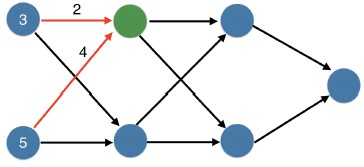
A round of backpropagation
In the network shown below, we have done forward propagation, and node values calculated as part of forward propagation are shown in white. The weights are shown in black. Layers after the question mark show the slopes calculated as part of back-prop, rather than the forward-prop values. Those slope values are shown in purple.
This network again uses the ReLU activation function, so the slope of the activation function is 1 for any node receiving a positive value as input. Assume the node being examined had a positive value (so the activation function's slope is 1).
What is the slope needed to update the weight with the question mark?

Possible Answers
0.2.6.
Not enough information.
Building deep learning models with keras
In this chapter, you'll use the Keras library to build deep learning models for both regression and classification. You'll learn about the Specify-Compile-Fit workflow that you can use to make predictions, and by the end of the chapter, you'll have all the tools necessary to build deep neural networks.
Creating a keras model
You've learned the theory of back-propagation, which is core to understanding deep learning. Now you'll learn how to create and optimize these networks using the Keras interface to the TensorFlow deep learning library.
Model building steps
The Keras workflow has 4 steps. First, you specify the architecture, which is things like: how many layers do you want? how many nodes in each layer? What activation function do you want to use in each layer? Next, you compile the model. This specifies the loss function, and some details about how optimization works. Then you fit the model. Which is that cycle of back-propagation and optimization of model weights with your data. And finally you will want to use your model to make predictions. We'll go through these steps sequentially. The first step is creating or specifying your model. - Specify Architecture - Compile - Fit - Predict
- Model specification
Here is the code to do that. This code has three blocks. First we import what we will need. Numpy is here only for reading some data. The other two imports are used for building our model. The second block of two lines reads the data. We read the data here so we can find the number of nodes in the input layer. That is stored as the variable n_cols. We always need to specify how many columns are in the input when building a keras model, because that is the number of nodes in the input layer. We then start building the model. The first line of model specification is model equals Sequential. There are two ways to build up a model, and we will focus on sequential, which is the easier way to build a model. Sequential models require that each layer has weights or connections only to the one layer coming directly after it in the network diagram. There are more exotic models out there with complex patterns of connections, but Sequential will do the trick for everything we need here. We start adding layers using the add method of the model. he type of layer you have seen, that standard layer type, is called a Dense layer. It is called Dense because all of the nodes in the previous layer connect to all of the nodes in the current layer. As you advance in deep learning, you may start using layers that aren't Dense. In each layer, we specify the number of nodes as the first positional argument, and the activation function we want to use in that layer using the keyword argument activation. Keras supports every activation function you will want in practice. In the first layer, we need to specify input shapes as shown here. That says the input will have n_cols columns, and there is nothing after the comma, meaning it can have any number of rows, that is, any number of data points. You'll notice the last layer has 1 node. That is the output layer, and it matches those diagrams where we ended with only a single node as the output or prediction of the model. This model has 2 hidden layers, and an output layer. You may be struck that each hidden layers has 100 nodes. Keras and TensorFlow do the math for us, so don't feel afraid to use much bigger networks than we've seen before. It's quite common to use 100 or 1000s nodes in a layer. You'll learn more about choosing an appropriate number of nodes later.
import numpy as np
from keras.layers import Dense
from keras.models import Sequential

predictors = np.loadtxt('predictors_data.csv', delimiter=',')
n_cols = predictors.shape[1]

model = Sequential()
model.add(Dense(100, activation='relu', input_shape=(n_cols,)))
model.add(Dense(100, activation='relu'))
model.add(Dense(1))
Understanding your data
You will soon start building models in Keras to predict wages based on various professional and demographic factors. Before you start building a model, it's good to understand your data by performing some exploratory analysis.
The data is pre-loaded into a pandas DataFrame called df. Use the .head() and .describe() methods in the IPython Shell for a quick overview of the DataFrame.
The target variable you'll be predicting is wage_per_hour. Some of the predictor variables are binary indicators, where a value of 1 represents True, and 0 represents False.
Of the 9 predictor variables in the DataFrame, how many are binary indicators? The min and max values as shown by .describe() will be informative here. How many binary indicator predictors are there?
Possible Answers
0.5.- 6.
# hourly_wages.csv
hw = pd.read_csv(data_paths[0])

display(hw.head(3))

hw.describe()
| wage_per_hour | union | education_yrs | experience_yrs | age | female | marr | south | manufacturing | construction | |
|---|---|---|---|---|---|---|---|---|---|---|
| 0 | 5.10 | 0 | 8 | 21 | 35 | 1 | 1 | 0 | 1 | 0 |
| 1 | 4.95 | 0 | 9 | 42 | 57 | 1 | 1 | 0 | 1 | 0 |
| 2 | 6.67 | 0 | 12 | 1 | 19 | 0 | 0 | 0 | 1 | 0 |
| wage_per_hour | union | education_yrs | experience_yrs | age | female | marr | south | manufacturing | construction | |
|---|---|---|---|---|---|---|---|---|---|---|
| count | 534.000000 | 534.000000 | 534.000000 | 534.000000 | 534.000000 | 534.000000 | 534.000000 | 534.000000 | 534.000000 | 534.000000 |
| mean | 9.024064 | 0.179775 | 13.018727 | 17.822097 | 36.833333 | 0.458801 | 0.655431 | 0.292135 | 0.185393 | 0.044944 |
| std | 5.139097 | 0.384360 | 2.615373 | 12.379710 | 11.726573 | 0.498767 | 0.475673 | 0.455170 | 0.388981 | 0.207375 |
| min | 1.000000 | 0.000000 | 2.000000 | 0.000000 | 18.000000 | 0.000000 | 0.000000 | 0.000000 | 0.000000 | 0.000000 |
| 25% | 5.250000 | 0.000000 | 12.000000 | 8.000000 | 28.000000 | 0.000000 | 0.000000 | 0.000000 | 0.000000 | 0.000000 |
| 50% | 7.780000 | 0.000000 | 12.000000 | 15.000000 | 35.000000 | 0.000000 | 1.000000 | 0.000000 | 0.000000 | 0.000000 |
| 75% | 11.250000 | 0.000000 | 15.000000 | 26.000000 | 44.000000 | 1.000000 | 1.000000 | 1.000000 | 0.000000 | 0.000000 |
| max | 44.500000 | 1.000000 | 18.000000 | 55.000000 | 64.000000 | 1.000000 | 1.000000 | 1.000000 | 1.000000 | 1.000000 |
Specifying a model
Now you'll get to work with your first model in Keras, and will immediately be able to run more complex neural network models on larger datasets compared to the first two chapters.
To start, you'll take the skeleton of a neural network and add a hidden layer and an output layer. You'll then fit that model and see Keras do the optimization so your model continually gets better.
As a start, you'll predict workers wages based on characteristics like their industry, education and level of experience. You can find the dataset in a pandas dataframe called df. For convenience, everything in df except for the target has been converted to a NumPy matrix called predictors. The target, wage_per_hour, is available as a NumPy matrix called target.
For all exercises in this chapter, we've imported the Sequential model constructor, the Dense layer constructor, and pandas.
Instructions
- Store the number of columns in the
predictorsdata ton_col. This has been done for you. - Start by creating a
Sequentialmodel calledmodel. - Use the
.add()method onmodelto add aDenselayer.- Add
50units, specifyactivation='relu', and theinput_shapeparameter to be the tuple(n_cols,)which means it hasn_colsitems in each row of data, and any number of rows of data are acceptable as inputs.
- Add
- Add another
Denselayer. This should have32units and a'relu'activation. - Finally, add an output layer, which is a
Denselayer with a single node. Don't use any activation function here.
# Import necessary modules
# import keras
# from keras.layers import Dense
# from keras.models import Sequential

predictors = hw.iloc[:, 1:].values

# Save the number of columns in predictors: n_cols
n_cols = predictors.shape[1]

# Set up the model: model
model = Sequential()

# Add the first layer
model.add(Dense(50, activation='relu', input_shape=(n_cols,)))

# Add the second layer
model.add(Dense(30, activation='relu'))

# Add the output layer
model.add(Dense(1))
Compiling and fitting a model
After you've specified a model, the next task is to compile it, which sets up the network for optimization, for instance creating an internal function to do back-propagation efficiently. The compile methods
Why you need to compile your model
has two important arguments for you to choose. The first is what optimizer to use, which controls the learning rate. In practice, the right choice of learning rate can make a big difference for how quickly our model finds good weights, and even how good a set of weights it can find. There are a few algorithms that automatically tune the learning rate. Even many experts in the field don't know all the details of all the optimization algorithms. So the pragmatic approach is to choose a versatile algorithm and use that for most problems. Adam is an excellent choice as your go-to optimizer. Adam adjusts the learning rate as it does gradient descent, to ensure reasonable values throughout the weight optimization process. The second thing you specify is the loss function. Mean squared error is the most common choice for regression problems. When we use keras for classification, you will learn a new default metric.
- Specify the optimizer
  - Many options and mathematically complex
  - "Adam" is usually a good choice
- Loss function
  - "mean_squared_error" common for regression
- Compiling a model
Here is an example of the code to compile a model. It builds a model, as you've already seen, and then we add a compile command after building the model. After compiling the model, you can
n_cols = predictors.shape[1]
model = Sequential()
model.add(Dense(100, activation='relu', input_shape = (n_cols,)))
model.add(Dense(100, activation='relu'))
model.add(Dense(1))
model.compile(optimizer='adam', loss='mean_squared_error')
- What is fitting a model
fit it. That is applying back-propagation and gradient descent with your data to update the weights. The fit step looks similar to what you've seen in scikit-learn, though it has more options which we will explore soon. Even with the Adam optimizer, which is pretty smart, it can improve your optimization process if you scale all the data so each feature is, on average, about similar sized values. One common approach is to subtract each feature by that features mean, and divide it by it's standard deviation.
 - Applying back-propagation and gradient descent with your data to update the weights
 - Scaling data before fitting can ease optimization
- Fitting a model
You can see what the code looks like here. After the compile step, we run fit, with the predictors as the first argument. When you run this, you will see some output showing the optimizations progress as it fits the data. We'll go into more detail about this output soon, but for now,
...
model.fit(predictors, target)
- Let's practice!
just think of it as a log showing model performance on the training data as we update model weights.
Compiling the model
You're now going to compile the model you specified earlier. To compile the model, you need to specify the optimizer and loss function to use. In the video, Dan mentioned that the Adam optimizer is an excellent choice. You can read more about it as well as other keras optimizers here, and if you are really curious to learn more, you can read the original paper that introduced the Adam optimizer.
In this exercise, you'll use the Adam optimizer and the mean squared error loss function. Go for it!
Instructions
Compile the model using
model.compile(). Youroptimizershould be'adam'and the loss should be'mean_squared_error'.
# Import necessary modules
# import keras
# from keras.layers import Dense
# from keras.models import Sequential

# Specify the model
n_cols = predictors.shape[1]
model = Sequential()
model.add(Dense(50, activation='relu', input_shape = (n_cols,)))
model.add(Dense(32, activation='relu'))
model.add(Dense(1))

# Compile the model
model.compile(optimizer='adam', loss='mean_squared_error')

# Verify that model contains information from compiling
print("Loss function: " + model.loss)
Loss function: mean_squared_error
Fitting the model
You're at the most fun part. You'll now fit the model. Recall that the data to be used as predictive features is loaded in a NumPy matrix called predictors and the data to be predicted is stored in a NumPy matrix called target. Your model is pre-written and it has been compiled with the code from the previous exercise.
Instructions
- Fit the
model. Remember that the first argument is the predictive features (predictors), and the data to be predicted (target) is the second argument.
# Import necessary modules
# import keras
# from keras.layers import Dense
# from keras.models import Sequential

target = hw.wage_per_hour.values

# Specify the model
n_cols = predictors.shape[1]
model = Sequential()
model.add(Dense(50, activation='relu', input_shape = (n_cols,)))
model.add(Dense(32, activation='relu'))
model.add(Dense(1))

# Compile the model
model.compile(optimizer='adam', loss='mean_squared_error')

# Fit the model
model.fit(x=predictors, y=target, epochs=5, verbose=1)
Epoch 1/5
17/17 [==============================] - 0s 2ms/step - loss: 30.3772
Epoch 2/5
17/17 [==============================] - 0s 1ms/step - loss: 22.7786
Epoch 3/5
17/17 [==============================] - 0s 1ms/step - loss: 21.8462
Epoch 4/5
17/17 [==============================] - 0s 1ms/step - loss: 21.4328
Epoch 5/5
17/17 [==============================] - 0s 1ms/step - loss: 21.2286
<tensorflow.python.keras.callbacks.History at 0x1e23df18940>
Classification models
- So far we have focused on regression models. But deep learning works similarly for classification, that is for predicting outcomes from a set of discrete options.
- Classification
For classification, you do a couple of things differently. The biggest changes are:1, set the loss function as 'categorical_crossentropy' instead of 'mean_squared_error'. This isn't the only possible loss function for classification problems, but it is by far the most common. You may have heard of this before under the name LogLoss. We won't go into the mathematics of categorical crossentropy here. For categorical crossentropy loss function, a lower score is better. But it's still hard to interpret. So I've added this argument "metrics equals accuracy". This means I want to print out the accuracy score at the end of each epoch, which makes it easier to see and understand the models progress. Second you need to modify the last layer, so it has a separate node for each potential outcome. You will also change the activation function to softmax. The softmax activation function ensures the predictions sum to 1, so they can be interpreted like probabilities.
- `categorical_crossentropy` loss function
- Similar to log loss: Lower is better
- Add `metrics=['accuracy']` to compile step for easy-to-understand diagnostics
- Output layer has separate node for each possible outcome, and uses `'softmax'` activation
- Quick look at the data
Here is some data for a binary classification problem. We have data from the NBA basketball league. It includes facts about each shot, and the
| shot_clock | dribbles | touch_time | shot_dis | close_def_dis | shot_result |
|---|---|---|---|---|---|
| 10.8 | 2 | 1.9 | 7.7 | 1.3 | 1 |
| 3.4 | 0 | 0.8 | 28.2 | 6.1 | 0 |
| 0 | 3 | 2.7 | 10.1 | 0.9 | 0 |
| 10.3 | 2 | 1.9 | 17.2 | 3.4 | 0 |
- Quick look at the data
shot result is either 0 or 1, indicating whether the shot went in or not. The outcome here is in a single column, which is not uncommon. But in general, we'll want to convert categoricals in Keras to a format with a separate column for each output. Keras includes a function to do that, which you will see in the code soon. This setup is consistent with the fact that your model will have a separate node in the output for each possible class.
- Transforming to categorical
We have a new column for each value of shot_result. A 1 in any column indicates that this column corresponds to the value from the original data. This is sometimes called one-hot encoding. If the original data had 3 or 4 or 100 different values, the new array for our data would have 3 or 4 or 100 columns respect
| shot_result | Outcome 0 | Outcome 1 | |
|---|---|---|---|
| 1 | → | 0 | 1 |
| 0 | → | 1 | 0 |
| 0 | → | 1 | 0 |
| 0 | → | 1 | 0 |
from tensorflow.keras.utils import to_categorical

data = pd.read_csv('basketball_shot_log.csv')
predictors = data.drop(['shot_result'], axis=1).values
target = to_categorical(data['shot_result'])

model = Sequential()
model.add(Dense(100, activation='relu', input_shape=(n_cols,)))
model.add(Dense(100, activation='relu'))
model.add(Dense(100, activation='relu'))
model.add(Dense(2, activation='softmax'))
model.compile(optimizer='adam', loss='categorical_crossentropy', metrics=['accuracy'])
model.fit(predictors, target)
- Classification
Lets look at the results now. Both accuracy and loss improve measurably for the first 3 epochs, and then the improvement slows down. Sometimes it gets a little worse for an epoch, sometimes it gets a little better. We will soon see a more sophisticated way to determine how long to train, but training for 10 epochs got us to that flat part of the loss function, so this worked well in this case.
Epoch 1/10 128069/128069 [==============================] - 4s - loss: 0.7706 - acc: 0.575
Epoch 2/10 128069/128069 [==============================] - 5s - loss: 0.6656 - acc: 0.003
Epoch 3/10 128069/128069 [==============================] - 6s - loss: 0.6611 - acc:0.6094
Epoch 4/10 128069/128069 [==============================] - 7s - loss: 0.6584 - ac: 0.6106
Epoch 5/10 128069/128069 [==============================] - 7s - loss: 0.6561 acc: 0.6150
Epoch 6/10 128069/128069 [==============================] - 9s - loss: 0.653 - acc: 0.6158
Epoch 7/10 128069/128069 [==============================] - 9s - loss: 06543 - acc: 0.6162
Epoch 8/10 128069/128069 [==============================] - 9s - loss 0.6538 - acc: 0.6158
Epoch 9/10 128069/128069 [==============================] - 10s - lss: 0.6535 - acc: 0.6157
Epoch 10/10 128069/128069 [==============================] - 10s loss: 0.6531 - acc: 0.6166
Understanding your classification data
Now you will start modeling with a new dataset for a classification problem. This data includes information about passengers on the Titanic. You will use predictors such as age, fare and where each passenger embarked from to predict who will survive. This data is from a tutorial on data science competitions. Look here for descriptions of the features.
The data is pre-loaded in a pandas DataFrame called df.
It's smart to review the maximum and minimum values of each variable to ensure the data isn't misformatted or corrupted. What was the maximum age of passengers on the Titanic? Use the .describe() method in the IPython Shell to answer this question.
Possible Answers
29.699.- 80.
891.It is not listed.
# titanic data
df = pd.read_csv(data_paths[2])
df.age_was_missing = df.age_was_missing.astype(int)  # convert Boolean to a number
display(df.head(2))
df.describe()
| survived | pclass | age | sibsp | parch | fare | male | age_was_missing | embarked_from_cherbourg | embarked_from_queenstown | embarked_from_southampton | |
|---|---|---|---|---|---|---|---|---|---|---|---|
| 0 | 0 | 3 | 22.0 | 1 | 0 | 7.2500 | 1 | 0 | 0 | 0 | 1 |
| 1 | 1 | 1 | 38.0 | 1 | 0 | 71.2833 | 0 | 0 | 1 | 0 | 0 |
| survived | pclass | age | sibsp | parch | fare | male | age_was_missing | embarked_from_cherbourg | embarked_from_queenstown | embarked_from_southampton | |
|---|---|---|---|---|---|---|---|---|---|---|---|
| count | 891.000000 | 891.000000 | 891.000000 | 891.000000 | 891.000000 | 891.000000 | 891.000000 | 891.000000 | 891.000000 | 891.000000 | 891.000000 |
| mean | 0.383838 | 2.308642 | 29.699118 | 0.523008 | 0.381594 | 32.204208 | 0.647587 | 0.198653 | 0.188552 | 0.086420 | 0.722783 |
| std | 0.486592 | 0.836071 | 13.002015 | 1.102743 | 0.806057 | 49.693429 | 0.477990 | 0.399210 | 0.391372 | 0.281141 | 0.447876 |
| min | 0.000000 | 1.000000 | 0.420000 | 0.000000 | 0.000000 | 0.000000 | 0.000000 | 0.000000 | 0.000000 | 0.000000 | 0.000000 |
| 25% | 0.000000 | 2.000000 | 22.000000 | 0.000000 | 0.000000 | 7.910400 | 0.000000 | 0.000000 | 0.000000 | 0.000000 | 0.000000 |
| 50% | 0.000000 | 3.000000 | 29.699118 | 0.000000 | 0.000000 | 14.454200 | 1.000000 | 0.000000 | 0.000000 | 0.000000 | 1.000000 |
| 75% | 1.000000 | 3.000000 | 35.000000 | 1.000000 | 0.000000 | 31.000000 | 1.000000 | 0.000000 | 0.000000 | 0.000000 | 1.000000 |
| max | 1.000000 | 3.000000 | 80.000000 | 8.000000 | 6.000000 | 512.329200 | 1.000000 | 1.000000 | 1.000000 | 1.000000 | 1.000000 |
Last steps in classification models
You'll now create a classification model using the titanic dataset, which has been pre-loaded into a DataFrame called df. You'll take information about the passengers and predict which ones survived.
The predictive variables are stored in a NumPy array predictors. The target to predict is in df.survived, though you'll have to manipulate it for keras. The number of predictive features is stored in n_cols.
Here, you'll use the 'sgd' optimizer, which stands for Stochastic Gradient Descent. You'll learn more about this in the next chapter!
Instructions
Convert
df.survivedto a categorical variable using theto_categorical()function.Specify a
Sequentialmodel calledmodel.Add a
Denselayer with32nodes. Use'relu'as theactivationand(n_cols,)as theinput_shape.Add the
Denseoutput layer. Because there are two outcomes, it should have 2 units, and because it is a classification model, theactivationshould be'softmax'.Compile the model, using
'sgd'as theoptimizer,'categorical_crossentropy'as the loss function, andmetrics=['accuracy']to see the accuracy (what fraction of predictions were correct) at the end of each epoch.Fit the model using the
predictorsand thetarget.
# Import necessary modules
# import keras
# from keras.layers import Dense
# from keras.models import Sequential
# from keras.utils import to_categorical

predictors = df.iloc[:, 1:].values
n_cols = predictors.shape[1]

# Convert the target to categorical: target
target = to_categorical(df.survived)
# Set up the model
model = Sequential()

# Add the first layer
model.add(Dense(32, activation='relu', input_shape=(n_cols,)))

# Add the output layer
model.add(Dense(2, activation='softmax'))

# Compile the model
model.compile(optimizer='sgd', loss='categorical_crossentropy', metrics=['accuracy'])

# Fit the model
model.fit(predictors, target, epochs=5, verbose=1)
Epoch 1/5
28/28 [==============================] - 0s 1ms/step - loss: 2.5361 - accuracy: 0.6218
Epoch 2/5
28/28 [==============================] - 0s 1ms/step - loss: 1.1159 - accuracy: 0.6330
Epoch 3/5
28/28 [==============================] - 0s 1ms/step - loss: 0.7131 - accuracy: 0.6891
Epoch 4/5
28/28 [==============================] - 0s 1ms/step - loss: 0.6187 - accuracy: 0.6790
Epoch 5/5
28/28 [==============================] - 0s 1ms/step - loss: 0.6200 - accuracy: 0.6902
<tensorflow.python.keras.callbacks.History at 0x1e4c09b5550>
Using models
Now that you can build basic deep learning models, I'll show you how to use them. Then we'll go into some finer details on fine tuning model architectures. The things you'll want to do in order to use these models are
- save a model after you've trained it
- reload that model
- make predictions with the model
Saving, reloading and using your Model
from tensorflow.keras.models import load_model
model.save('model_file.h5')
my_model = load_model('model_file.h5')
predictions = my_model.predict(data_to_predict_with)
probability_true = predictions[:, 1]
- Here is the code to save a model, reload it, and make predictions. We've imported a
load_modelfunction here. Once I have a model I want to save, I can save it with thesavemethod. I supply a filename. Models are saved in a format called hdf5, for which h5 is the common extension. I then load the model back into memory with theload_modelfunction here. I then make predictions. The model I've loaded here is a classification model. The predictions come in the same format as the prediction target. You may recall that this had 1 column for whether the shot was missed, and then a 2nd column for whether the shot was made. In practice, I probably only want the probability that the shot is made. So, I'll extract that second column withnumpyindexing, and I called thatprobability_true. Lastly, sometimes I'll want to verify that the model I loaded has the same structure I expect.
Verifying model structure
- You can print out a summary of the model architecture with the
summarymethod. You can see the output here. Now that you can save your model, reload it, make predictions, and verify its structure, you have most of what you need to not just build models, but to work with them in practical situations. 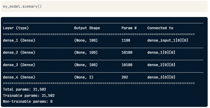
- You can print out a summary of the model architecture with the
Making predictions
The trained network from your previous coding exercise is now stored as model. New data to make predictions is stored in a NumPy array as pred_data. Use model to make predictions on your new data.
In this exercise, your predictions will be probabilities, which is the most common way for data scientists to communicate their predictions to colleagues.
Instructions
- Create your predictions using the model's
.predict()method onpred_data. - Use NumPy indexing to find the column corresponding to predicted probabilities of survival being True. This is the second column (index
1) ofpredictions. Store the result inpredicted_prob_trueand print it.
# Specify, compile, and fit the model
model = Sequential()
model.add(Dense(32, activation='relu', input_shape=(n_cols,)))
model.add(Dense(2, activation='softmax'))
model.compile(optimizer='sgd',
              loss='categorical_crossentropy',
              metrics=['accuracy'])

model.fit(predictors[:800, :], target[:800, :])

# Calculate predictions: predictions
pred_data = predictors[800:, :]
predictions = model.predict(pred_data)

# Calculate predicted probability of survival: predicted_prob_true
predicted_prob_true = predictions[:, 1]

# Print predicted_prob_true
predicted_prob_true
25/25 [==============================] - 0s 1ms/step - loss: 2.1631 - accuracy: 0.5562
array([0.14567937, 0.18335524, 0.990599  , 0.7644454 , 0.20688732,
       0.16710629, 0.02948781, 0.32653692, 0.10595483, 0.34744728,
       0.22476563, 0.1340201 , 0.12653537, 0.7111234 , 0.17362803,
       0.05378632, 0.25303987, 0.29152656, 0.07391907, 0.5541538 ,
       0.26096934, 0.21695887, 0.03222005, 0.21665907, 0.8414357 ,
       0.17796974, 0.40962723, 0.90199107, 0.18228547, 0.21002501,
       0.38249457, 0.75846094, 0.17792921, 0.26488808, 0.34510124,
       0.36842877, 0.3003544 , 0.17345351, 0.45608845, 0.23062544,
       0.31014034, 0.3439002 , 0.26858   , 0.13600093, 0.36479202,
       0.08198298, 0.23487027, 0.13783525, 0.32359642, 0.70273167,
       0.76990974, 0.00844374, 0.5318753 , 0.53725845, 0.09431058,
       0.32170808, 0.96364856, 0.05290617, 0.2508271 , 0.17792921,
       0.12100039, 0.30353713, 0.05930348, 0.22118652, 0.24584311,
       0.08197409, 0.22468218, 0.40365848, 0.1811305 , 0.6053713 ,
       0.22482468, 0.18244971, 0.10741129, 0.06134324, 0.22722283,
       0.38229367, 0.32472122, 0.32566735, 0.17256665, 0.29156753,
       0.31471428, 0.14831473, 0.28564858, 0.19433397, 0.23238342,
       0.11268502, 0.21445668, 0.42943263, 0.20138258, 0.31850585,
       0.16675813], dtype=float32)
Fine-tuning keras models
Learn how to optimize your deep learning models in Keras. Start by learning how to validate your models, then understand the concept of model capacity, and finally, experiment with wider and deeper networks.
Understanding model optimization
- At this point, you have a good understanding of how neural networks work, and how to build them in Keras. But you probably don't yet have a great intuition for how to choose things like model architecture and model optimization arguments. You'll learn that in this last chapter.
- Why optimization is hard
In practice, optimization is a hard problem. The optimal value for any one weight depends on the values of the other weights, and we are optimizing many weights at once. Even if the slope tells us which weights to increase, and which to decrease, our updates may not improve our model meaningfully. A small learning rate might cause us to make such small updates to the model's weights that our model doesn't improve materially. A very large learning rate might take us too far in the direction that seemed good. A smart optimizer like Adam helps, but optimization problems can still occur. The easiest way to see the effect of different learning rates is to use the simplest optimizer,
- Simultaneously optimizing 1000s of parameters with complex relationships
- Updates may not improve model meaningfully
- Updates too small (if learning rate is slow) or too large (if learning rate is high)
- Stochastic gradient descent
Stochastic Gradient Descent, sometimes abbreviated to SGD. This optimizer uses a fixed learning rate. Learning rates around point-01 are common. But you can specify the learning rate you need with lr argument as shown here. We have a function that creates a new model here. We create models in a for loop, and each time around we compile the model using SGD with a different learning rate. We pass in the optimizer with the same argument where we previously passed the string for "Adam". In an exercise, you will compare the results of training models trained with low, medium and high learning rates. Even if your learning rate is well tuned, you can run into the so-called
- The dying neuron problem
"dying-neuron" problem. This problem occurs when a neuron takes a value less than 0 for all rows of your data. Recall that, with the ReLU activation function, any node with a negative input value produces an output of 0, and it also has a slope of 0 as you see in this graph. Because the slope is 0, the slope of any weights flowing into that node are also 0. So those weights don't get updated. In other words, once the node starts always getting negative inputs, it may continue only getting negative inputs. It's contributing nothing to the model at this point, and hence the claim that the node or neuron is "dead." At first, this might suggest using an activation function whose slope is never exactly zero. However, those types of functions were used for many years.
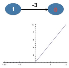
- Vanishing gradients
For example, in an earlier video we used an s-shaped function called tanh. However, values that were outside the middle of the S were
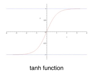
- Vanishing gradients
relatively flat, or had small slopes. A small but non-zero slope might work in a network with only a few hidden layers. But in a deep network, one with many layers, the repeated multiplication of small slopes causes the slopes to get close to 0, which meant updates in backprop were close to 0. This is called the vanishing gradient problem. This in turn might suggest using an activation function that isn't even close to flat anywhere. There is research in this area, including variations on ReLU. Those aren't widely used though. For now, it's a phenomenon worth keeping in mind if you are ever pondering why your model isn't training better. If it happens, changing the activation function may be the solution.
- Occurs when many layers have very small slopes (e.g. due to being on flat part of tanh curve
- In deep networks, updates to backprop were close to 0
def get_new_model
def get_new_model(input_shape):
    model = Sequential()
    model.add(Dense(100, activation='relu', input_shape=input_shape))
    model.add(Dense(100, activation='relu'))
    model.add(Dense(2, activation='softmax'))
    return model
lr_to_test = [0.000001, 0.01, 1]

# loop over learning rates
for lr in lrt_to_test:
    model = get_new_model()
    my_optimizer = SGD(lr=lr)
    model.compile(optimizer=my_optimizer, loss='categorical_crossentropy')
    model.fit(predictors, target)
Diagnosing optimization problems
Which of the following could prevent a model from showing an improved loss in its first few epochs?
Answer the question
Learning rate too lowLearning rate too highPoor choice of activation function- All of the above
Changing optimization parameters
It's time to get your hands dirty with optimization. You'll now try optimizing a model at a very low learning rate, a very high learning rate, and a "just right" learning rate. You'll want to look at the results after running this exercise, remembering that a low value for the loss function is good.
For these exercises, we've pre-loaded the predictors and target values from your previous classification models (predicting who would survive on the Titanic). You'll want the optimization to start from scratch every time you change the learning rate, to give a fair comparison of how each learning rate did in your results. So we have created a function get_new_model() that creates an unoptimized model to optimize.
Instructions
- Import
SGDfromkeras.optimizers. - Create a list of learning rates to try optimizing with called
lr_to_test. The learning rates in it should be.000001,0.01, and1. - Using a
forloop to iterate overlr_to_test:- Use the
get_new_model()function to build a new, unoptimized model. - Create an optimizer called
my_optimizerusing theSGD()constructor with keyword argumentlr=lr. - Compile your model. Set the optimizer parameter to be the SGD object you created above, and because this is a classification problem, use
'categorical_crossentropy'for thelossparameter. - Fit your model using the
predictorsandtarget.
- Use the
# setup data
# titanic data
df = pd.read_csv(data_paths[2])
df.age_was_missing = df.age_was_missing.astype(int)  # convert Boolean to a number

predictors = df.iloc[:, 1:].values
n_cols = predictors.shape[1]
input_shape = (n_cols,)

# Convert the target to categorical: target
target = to_categorical(df.survived)
# Import the SGD optimizer, which is done in the Imports section
# from tensorflow.keras.optimizers import SGD

# Create list of learning rates: lr_to_test
lr_to_test = [0.000001, 0.01, 0.1]

# Loop over learning rates
for lr in lr_to_test:
    print('\n\nTesting model with learning rate: %f\n'%lr )

    # Build new model to test, unaffected by previous models
    model = get_new_model(input_shape)

    # Create SGD optimizer with specified learning rate: my_optimizer
    my_optimizer = SGD(learning_rate=lr)

    # Compile the model
    model.compile(optimizer=my_optimizer, loss='categorical_crossentropy')

    # Fit the model
    model.fit(predictors, target)
Testing model with learning rate: 0.000001

28/28 [==============================] - 0s 1ms/step - loss: 4.9162


Testing model with learning rate: 0.010000

28/28 [==============================] - 0s 1ms/step - loss: 1.7546


Testing model with learning rate: 0.100000

28/28 [==============================] - 0s 1ms/step - loss: 5.9029
Model validation
You may recall from previous machine learning classes that your model's performance on the training data is not a good indication of how it will perform on new data. For this reason, we use validation data to test model performance. Validation data is data that is explicitly held out from training, and used only to test model performance.
Validation in deep learning
You may already be familiar with k-fold cross validation. In practice, few people run k-fold cross validation on deep learning models because deep learning is typically used on large datasets. So the computational expense of running k-fold validation would be large, and we usually trust a score from a single validation run because those validation runs are reasonably large. Keras makes it easy to use some of your data as validation data, and we see that
- Commonly use validation split rather than cross-validation
- Deep learning widely used on large datasets
- Single validation score is based on large amount of data, and is reliable
- Model validation
in this code, where we specify the split using the keyword argument validation_split when calling the fit method. Here, we have already specified a model, and we'll make small changes in both the compile and fit steps to see model validation information. This is a classification problem, and we'd like to see measures of accuracy. So, we include metrics equals 'accuracy' in the compile step. In the fit step, we specify what fraction of the data is used for validation. In this case, we'll use 30%.Our goal is to have the best validation score possible, so we should keep training while validation score is improving, and then stop training when the validation score isn't improving. We do this with something called
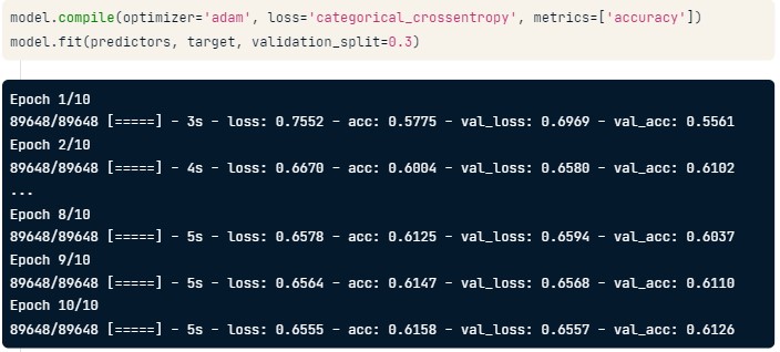
- Early Stopping
"early stopping." We can use early stopping with only some small changes to the code. See here, we've imported something called EarlyStopping. We then create an "early stopping monitor" before fitting the model. That monitor takes an argument called patience, which is how many epochs the model can go without improving before we stop training. 2 or 3 are reasonable values for patience. Sometimes you'll get a single epoch with no improvement, but the model will start improving again after that epoch. But if you see 3 epochs with no improvement, it's unlikely to turn around and start improving again. We pass early_stopping_monitor to the fit function under an argument called callbacks. Notice that callbacks takes a list. You may consider adding other callbacks as you become very advanced. But early stopping is all you want for now. By default, keras trains for 10 epochs. Now that we have smart logic for determining when to stop, we can set a high maximum number of epochs. This happens with the nb_epoch argument, as you see here. Keras will go until this number of epochs, unless the validation loss stops improving, in which case it will stop earlier. This is smarter training logic than relying on a fixed number of epochs without looking at the validation scores.
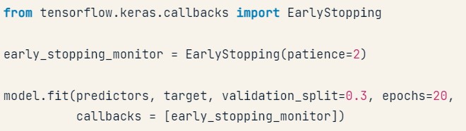
- Output from early stopping
Let's look at the output. In epoch 9 we had a validation loss score of point-6513. We didn't beat that score in the next 2 epochs, so we stopped training. Now that you have a reliable way of measuring model performance, namely through scores, you should feel free
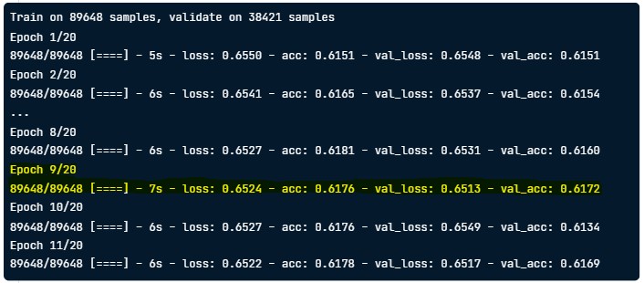
- Experimentation
to experiment with different architectures. More layers, fewer layers. Layers with more nodes, layers with fewer nodes. And so on. Creating a great model requires some experimentation. Before we finish, we'll give a little bit of insight into how to choose where you experiment.
- More layers
- Fewer layers
- Layers with more nodes
- Layers with fewer nodes
- Creating a great model requires experimentation
- Let's practice!
But, now that you can get validation scores, you are poised to run those experiments and figure out what works best for your data.
Evaluating model accuracy on validation dataset
Now it's your turn to monitor model accuracy with a validation data set. A model definition has been provided as model. Your job is to add the code to compile it and then fit it. You'll check the validation score in each epoch.
Instructions
- Compile your model using
'adam'as theoptimizerand'categorical_crossentropy'for theloss. To see what fraction of predictions are correct (theaccuracy) in each epoch, specify the additional keyword argumentmetrics=['accuracy']inmodel.compile(). - Fit the model using the
predictorsandtarget. Create a validation split of 30% (or0.3). This will be reported in each epoch.
# Save the number of columns in predictors: n_cols
n_cols = predictors.shape[1]
input_shape = (n_cols,)

# Specify the model
model = Sequential()
model.add(Dense(100, activation='relu', input_shape=input_shape))
model.add(Dense(100, activation='relu'))
model.add(Dense(2, activation='softmax'))

# Compile the model
model.compile(optimizer='adam', loss='categorical_crossentropy', metrics=['accuracy'])

# Fit the model
hist = model.fit(predictors, target, validation_split=0.3)
20/20 [==============================] - 0s 8ms/step - loss: 0.8591 - accuracy: 0.6453 - val_loss: 0.7441 - val_accuracy: 0.6642
Early stopping: Optimizing the optimization
Now that you know how to monitor your model performance throughout optimization, you can use early stopping to stop optimization when it isn't helping any more. Since the optimization stops automatically when it isn't helping, you can also set a high value for epochs in your call to .fit(), as Dan showed in the video.
The model you'll optimize has been specified as model. As before, the data is pre-loaded as predictors and target.
Instructions
- Import
EarlyStoppingfromtensorflow.keras.callbacks. - Compile the model, once again using
'adam'as theoptimizer,'categorical_crossentropy'as the loss function, andmetrics=['accuracy']to see the accuracy at each epoch. - Create an
EarlyStoppingobject calledearly_stopping_monitor. Stop optimization when the validation loss hasn't improved for 2 epochs by specifying thepatienceparameter ofEarlyStopping()to be2. - Fit the model using the
predictorsandtarget. Specify the number ofepochsto be30and use a validation split of0.3. In addition, pass[early_stopping_monitor]to thecallbacksparameter.
# Import EarlyStopping
# from tensorflow.keras.callbacks import EarlyStopping

# Save the number of columns in predictors: n_cols
n_cols = predictors.shape[1]
input_shape = (n_cols,)

# Specify the model
model = Sequential()
model.add(Dense(100, activation='relu', input_shape=input_shape))
model.add(Dense(100, activation='relu'))
model.add(Dense(2, activation='softmax'))

# Compile the model
model.compile(optimizer='adam', loss='categorical_crossentropy', metrics=['accuracy'])

# Define early_stopping_monitor
early_stopping_monitor = EarlyStopping(patience=2)

# Fit the model
hist = model.fit(predictors, target, validation_split=0.3, epochs=30, callbacks=[early_stopping_monitor])
Epoch 1/30
20/20 [==============================] - 0s 7ms/step - loss: 1.0995 - accuracy: 0.6067 - val_loss: 1.0541 - val_accuracy: 0.3545
Epoch 2/30
20/20 [==============================] - 0s 3ms/step - loss: 0.7416 - accuracy: 0.6100 - val_loss: 0.6975 - val_accuracy: 0.6493
Epoch 3/30
20/20 [==============================] - 0s 3ms/step - loss: 0.6284 - accuracy: 0.6918 - val_loss: 0.6053 - val_accuracy: 0.6791
Epoch 4/30
20/20 [==============================] - 0s 3ms/step - loss: 0.6310 - accuracy: 0.6790 - val_loss: 0.5499 - val_accuracy: 0.7575
Epoch 5/30
20/20 [==============================] - 0s 3ms/step - loss: 0.6026 - accuracy: 0.6918 - val_loss: 0.5236 - val_accuracy: 0.7537
Epoch 6/30
20/20 [==============================] - 0s 3ms/step - loss: 0.6084 - accuracy: 0.7030 - val_loss: 0.6164 - val_accuracy: 0.7052
Epoch 7/30
20/20 [==============================] - 0s 3ms/step - loss: 0.5811 - accuracy: 0.7030 - val_loss: 0.6076 - val_accuracy: 0.6604
Wonderful work! Because optimization will automatically stop when it is no longer helpful, it is okay to specify the maximum number of epochs as 30 rather than using the default of 10 that you've used so far. Here, it seems like the optimization stopped after 4 epochs.
Experimenting with wider networks
Now you know everything you need to begin experimenting with different models!
A model called model_1 has been pre-loaded. You can see a summary of this model printed in the IPython Shell. This is a relatively small network, with only 10 units in each hidden layer.
In this exercise you'll create a new model called model_2 which is similar to model_1, except it has 100 units in each hidden layer.
After you create model_2, both models will be fitted, and a graph showing both models loss score at each epoch will be shown. We added the argument verbose=False in the fitting commands to print out fewer updates, since you will look at these graphically instead of as text.
Because you are fitting two models, it will take a moment to see the outputs after you hit run, so be patient.
Instructions
- Create
model_2to replicatemodel_1, but use100nodes instead of10for the first twoDenselayers you add with the'relu'activation. Use2nodes for theDenseoutput layer with'softmax'as theactivation. - Compile
model_2as you have done with previous models: Using'adam'as theoptimizer,'categorical_crossentropy'for the loss, andmetrics=['accuracy']. - Hit 'Submit Answer' to fit both the models and visualize which one gives better results! Notice the keyword argument
verbose=Falseinmodel.fit(): This prints out fewer updates, since you'll be evaluating the models graphically instead of through text.
# Specify the model
model_1 = Sequential()
model_1.add(Dense(10, activation='relu', input_shape=input_shape))
model_1.add(Dense(10, activation='relu'))
model_1.add(Dense(2, activation='softmax'))

# Compile the model
model_1.compile(optimizer='adam', loss='categorical_crossentropy', metrics=['accuracy'])

model_1.summary()
Model: "sequential_10"
_________________________________________________________________
Layer (type)                 Output Shape              Param #
=================================================================
dense_28 (Dense)             (None, 10)                110
_________________________________________________________________
dense_29 (Dense)             (None, 10)                110
_________________________________________________________________
dense_30 (Dense)             (None, 2)                 22
=================================================================
Total params: 242
Trainable params: 242
Non-trainable params: 0
_________________________________________________________________
# Define early_stopping_monitor
early_stopping_monitor = EarlyStopping(patience=2)

# Create the new model: model_2
model_2 = Sequential()

# Add the first and second layers
model_2.add(Dense(100, activation='relu', input_shape=input_shape))
model_2.add(Dense(100, activation='relu'))

# Add the output layer
model_2.add(Dense(2, activation='softmax'))

# Compile model_2
model_2.compile(optimizer='adam', loss='categorical_crossentropy', metrics=['accuracy'])

# Fit model_1
model_1_training = model_1.fit(predictors, target, epochs=15, validation_split=0.2, callbacks=[early_stopping_monitor], verbose=False)

# Fit model_2
model_2_training = model_2.fit(predictors, target, epochs=15, validation_split=0.2, callbacks=[early_stopping_monitor], verbose=False)
# Create the plot
plt.plot(model_1_training.history['val_loss'], 'r', label='model_1')
plt.plot(model_2_training.history['val_loss'], 'b', label='model_2')
plt.xlabel('Epochs')
plt.ylabel('Validation score')
_ = plt.legend()

The blue model is the one you made, the red is the original model. Your model had a lower loss value, so it is the better model. Nice job!
Adding layers to a network
You've seen how to experiment with wider networks. In this exercise, you'll try a deeper network (more hidden layers).
Once again, you have a baseline model called model_1 as a starting point. It has 1 hidden layer, with 10 units. You can see a summary of that model's structure printed out. You will create a similar network with 3 hidden layers (still keeping 10 units in each layer).
This will again take a moment to fit both models, so you'll need to wait a few seconds to see the results after you run your code.
Instructions
- Specify a model called
model_2that is likemodel_1, but which has 3 hidden layers of 50 units instead of only 1 hidden layer.- Use
input_shapeto specify the input shape in the first hidden layer. - Use
'relu'activation for the 3 hidden layers and'softmax'for the output layer, which should have 2 units.
- Use
- Compile
model_2as you have done with previous models: Using'adam'as theoptimizer,'categorical_crossentropy'for theloss, andmetrics=['accuracy']. - Hit 'Submit Answer' to fit both the models and visualize which one gives better results! For both models, you should look for the best val_loss and val_acc, which won't be the last epoch for that model.
# Specify the model
model_1 = Sequential()
model_1.add(Dense(10, activation='relu', input_shape=input_shape))
model_1.add(Dense(2, activation='softmax'))

# Compile the model
model_1.compile(optimizer='adam', loss='categorical_crossentropy', metrics=['accuracy'])

model_1.summary()
Model: "sequential_12"
_________________________________________________________________
Layer (type)                 Output Shape              Param #
=================================================================
dense_34 (Dense)             (None, 10)                110
_________________________________________________________________
dense_35 (Dense)             (None, 2)                 22
=================================================================
Total params: 132
Trainable params: 132
Non-trainable params: 0
_________________________________________________________________
# The input shape to use in the first hidden layer
input_shape = (n_cols,)

# Create the new model: model_2
model_2 = Sequential()

# Add the first, second, and third hidden layers
model_2.add(Dense(10, activation='relu', input_shape=input_shape))
model_2.add(Dense(10, activation='relu'))
model_2.add(Dense(10, activation='relu'))

# Add the output layer
model_2.add(Dense(2, activation='softmax'))

# Compile model_2
model_2.compile(optimizer='adam', loss='categorical_crossentropy', metrics=['accuracy'])

# Fit model 1
model_1_training = model_1.fit(predictors, target, epochs=20, validation_split=0.4, callbacks=[early_stopping_monitor], verbose=False)

# Fit model 2
model_2_training = model_2.fit(predictors, target, epochs=20, validation_split=0.4, callbacks=[early_stopping_monitor], verbose=False)
# Create the plot
plt.plot(model_1_training.history['val_loss'], 'r', label='model_1')
plt.plot(model_2_training.history['val_loss'], 'b', label='model_2')
plt.xlabel('Epochs')
plt.ylabel('Validation score')
_ = plt.legend()

Great work! The blue model is the one you made and the red is the original model. The model with the lower loss value is the better model.
Thinking about model capacity
At this point, you know how to run experiments, and compare different models performance. However, it takes some practice to get an intuition for what experiments or architectures to try. There is still a little more art to finding good deep learning architectures than there is for tuning other machine learning algorithms. But something called "model capacity" should be one of the key considerations you think about when deciding what models to try."Model capacity" or "network capacity" is closely related to the terms overfitting and underfitting.
Overfitting
You may recall overfitting and a graphic like this from a previous DataCamp course. Overfitting is the ability of a model to fit oddities in your training data that are there purely due to happenstance, and that won't apply in a new dataset.
- When you are overfitting, your model will make accurate predictions on training data, but it will make inaccurate predictions on validation data and new datasets.
- Underfitting is the opposite. That is when your model fails to find important predictive patterns in the training data. So it is accurate in neither the training data nor validation data.
- Because we want to do well on new datasets that weren't used for training the model, our validation score is the ultimate measure of a model's predictive quality.
- Let's get back to model capacity. Model capacity is a model's ability to capture predictive patterns in your data. So, the more capacity a model, the further to the right we will be on this graph. If you had a network, and you increased the number of nodes or neurons in a hidden layer, that would increase model capacity. And if you add layers, that increases capacity. Said another way, making larger layers or increasing the number of layers moves you further to the right of this graph. So, with that in mind,
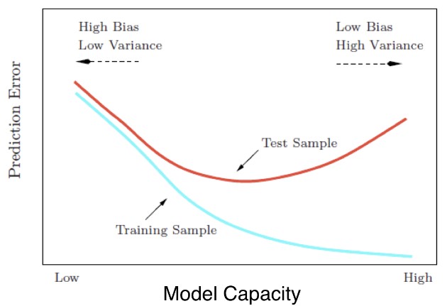
- Workflow for optimizing model capacity
here is a good workflow for you. Start with a simple network, and get the validation score. Then keep adding capacity as long as the score keeps improving. Once it stops improving, you can decrease capacity slightly, but you are probably near the ideal.
- Start with a small network
- Gradually increase capacity
- Keep increasing capacity until validation score is no longer improving
- Sequential experiments
Let's walk through that process once. Here, I've started a model that has one hidden layer and 100 units. That's a relatively simple, or low capacity, model. I get a mean squared error
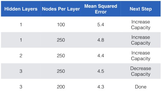
- Sequential experiments
of 5-point-4. Since I started with a simple model, I now try increasing capacity. I could increase the number of layers or use more hidden nodes. I'll start by using more nodes in the one hidden layer. That improved the model, so I'll keep increasing capacity.
- Sequential experiments
This time I'll switch to using 2 hidden layers. Each layer has 250 nodes. That improved the error more. So, I try 3 layers, continuing to add capacity as long as it helps.
- Sequential experiments
This hurt the score. So, the model with 2 layers and 250 nodes is about perfect. I'll try another model that reduces capacity slightly from the last model I built.
- Sequential experiments
That is 3 hidden layers with 200 nodes each. That seems the best model yet. So I'll stick with that. Should you change capacity by adding layers or by adding nodes to an existing layer? There isn't a universal answer to that. You can experiment. But you should generally be thinking about whether you are trying to increase or decrease capacity, ideally honing in on the right capacity by looking at validation scores.
Experimenting with model structures
You've just run an experiment where you compared two networks that were identical except that the 2nd network had an extra hidden layer. You see that this 2nd network (the deeper network) had better performance. Given that, which of the following would be a good experiment to run next for even better performance?
Answer the question
Try a new network with fewer layers than anything you have tried yet.- Use more units in each hidden layer.
Use fewer units in each hidden layer.
Stepping up to images
To close, you are going to apply your knowledge to a new and different dataset.
Recognizing handwritten digits
This is the MNIST dataset, which contains images of handwritten digits. This is a very popular dataset for getting started working with images. There is an image of each handwritten digit, and each image is composed of a 28 pixel by 28 pixel grid. The image is represented by showing how dark each pixel is. So, 0 would be as light as possible, and 255 is as dark as possible. I've flattened the 28 x 28 grid for you into a 784 x 1 array for each image. Each image shows a digit like 0, 1, 2, 3, 4, all the way up to 9. Your model will predict which digit it is that was written. So you will create a deep learning model taking in those 784 features for each image as inputs, and predicting digits from among 10 possible values for the output.
Building your own digit recognition model
You've reached the final exercise of the course - you now know everything you need to build an accurate model to recognize handwritten digits!
We've already done the basic manipulation of the MNIST dataset shown in the video, so you have X and y loaded and ready to model with. Sequential and Dense from tensorflow.keras are also pre-imported.
To add an extra challenge, we've loaded only 2500 images, rather than 60000 which you will see in some published results. Deep learning models perform better with more data, however, they also take longer to train, especially when they start becoming more complex.
If you have a computer with a CUDA compatible GPU, you can take advantage of it to improve computation time. If you don't have a GPU, no problem! You can set up a deep learning environment in the cloud that can run your models on a GPU. Here is a blog post by Dan that explains how to do this - check it out after completing this exercise! It is a great next step as you continue your deep learning journey.
Ready to take your deep learning to the next level? Check out Advanced Deep Learning with Keras to see how the Keras functional API lets you build domain knowledge to solve new types of problems. Once you know how to use the functional API, take a look at Image Processing with Keras in Python to learn image-specific applications of Keras..
Instructions
- Create a Sequential object to start your model. Call this model.
- Add the first
Densehidden layer of50units to your model with'relu'activation. For this data, theinput_shapeis(784,). - Add a second
Densehidden layer with50units and a'relu'activation function. - Add the output layer. Your activation function should be
'softmax', and the number of nodes in this layer should be the same as the number of possible outputs in this case:10. - Compile
modelas you have done with previous models: Using'adam'as theoptimizer,'categorical_crossentropy'for theloss, andmetrics=['accuracy']. - Fit the model using
Xandyusing avalidation_splitof0.3.
from tensorflow.keras.datasets import mnist
(x_train, y_train), (x_test, y_test) = mnist.load_data()
assert x_train.shape == (60000, 28, 28)
assert x_test.shape == (10000, 28, 28)
assert y_train.shape == (60000,)
assert y_test.shape == (10000,)
X = x_test.reshape((10000, 784))
y = np.zeros((y_test.size, y_test.max() + 1))
y[np.arange(y_test.size), y_test] = 1
y[0]
array([0., 0., 0., 0., 0., 0., 0., 1., 0., 0.])
y_test[0]
7
# Create the model: model
model = Sequential()

# Add the first hidden layer
model.add(Dense(50, activation='relu', input_shape=(784,)))

# Add the second hidden layer
model.add(Dense(50, activation='relu'))

# Add the output layer
model.add(Dense(10, activation='softmax'))

# Compile the model
model.compile(optimizer='adam', loss='categorical_crossentropy', metrics=['accuracy'])

# Fit the model
model.fit(X, y, epochs=10, validation_split=0.3)
Epoch 1/10
219/219 [==============================] - 1s 3ms/step - loss: 6.9723 - accuracy: 0.6180 - val_loss: 1.7533 - val_accuracy: 0.7673
Epoch 2/10
219/219 [==============================] - 1s 2ms/step - loss: 1.4124 - accuracy: 0.7709 - val_loss: 1.0788 - val_accuracy: 0.8153
Epoch 3/10
219/219 [==============================] - 1s 2ms/step - loss: 0.8167 - accuracy: 0.8190 - val_loss: 0.9107 - val_accuracy: 0.8277
Epoch 4/10
219/219 [==============================] - 1s 2ms/step - loss: 0.5930 - accuracy: 0.8547 - val_loss: 0.8294 - val_accuracy: 0.8377
Epoch 5/10
219/219 [==============================] - 1s 2ms/step - loss: 0.4901 - accuracy: 0.8699 - val_loss: 0.8243 - val_accuracy: 0.8493
Epoch 6/10
219/219 [==============================] - 1s 2ms/step - loss: 0.4056 - accuracy: 0.8911 - val_loss: 0.7467 - val_accuracy: 0.8567
Epoch 7/10
219/219 [==============================] - 1s 2ms/step - loss: 0.3549 - accuracy: 0.9054 - val_loss: 0.5833 - val_accuracy: 0.8727
Epoch 8/10
219/219 [==============================] - 1s 2ms/step - loss: 0.2733 - accuracy: 0.9204 - val_loss: 0.6773 - val_accuracy: 0.8717
Epoch 9/10
219/219 [==============================] - 1s 2ms/step - loss: 0.2872 - accuracy: 0.9203 - val_loss: 0.7157 - val_accuracy: 0.8763
Epoch 10/10
219/219 [==============================] - 1s 2ms/step - loss: 0.2614 - accuracy: 0.9264 - val_loss: 0.6382 - val_accuracy: 0.8947
<tensorflow.python.keras.callbacks.History at 0x1e21f49c850>
Final Thoughts
Congrats. You are on your way to using the most fun and powerful modeling technique around.
Next steps - There is still an immense amount to learn as you become a deep learning master. But it's like riding a bike. The hardest part is getting to the point where you can practice on your own, and you are there. You'll probably enjoy experimenting with deep learning using the same types of data you've used before for predictive modeling, tables of numeric data like what you commonly see in a pandas DataFrame or numpy array. From there, many people start working with images, using something called convolutional neural networks. But you could decide you want to focus on text. Or sound. Or you might get creative and apply deep learning to data others haven't even thought of. You'll find it's a powerful technique as you get the hang of it. Kaggle is a great place to find datasets to work with, and their forums are a great place to keep learning. As you get more advanced, start checking out the wikipedia page titled "List of datasets for machine learning research." It includes datasets from some very interesting domains. Keras has excellent documentation. When there's something specific to look up, keras-dot-io is likely to have the answer. The keras and tensorflow repositories on github also have nice examples to work from. As you start working with larger datasets and more complex deep learning models, you may find these models can take a long time to fit. If you have a computer with a graphical processing unit, or GPU, you may be able to set up TensorFlow to use that GPU for computation. This generally requires a GPU that meets a standard called CUDA compatibility. Most GPU's made by NVIDIA are CUDA compatible. If you don't have a computer with a CUDA compatible GPU, here is a link with instructions about setting up a deep learning environment in the cloud that can run your models on a GPU. More than anything, share your work online, and have fun. If you keep experimenting and build out on the tools you've learned, you'll soon be amazed at what you can do.
- Start with standard prediction problems on tables of numbers
- Images (with convolutional neural networks) are common next steps
- keras.io for excellent documentation
- Graphical processing unit (GPU) provides dramatic speedups in model training times
- Need a CUDA compatible GPU
- FOr training on GPUs in the cloud look here:
Certificate