1
2
3
4
5
6
| import pandas as pd
import matplotlib.pyplot as plt
import numpy as np
import seaborn as sns
from statsmodels.graphics.mosaicplot import mosaic
import statsmodels.formula.api as sm
|
1
2
3
4
| pd.set_option('display.max_columns', 700)
pd.set_option('display.max_rows', 400)
pd.set_option('display.min_rows', 20)
pd.set_option('display.expand_frame_repr', True)
|
1
2
3
4
5
6
7
| titanic_df = sns.load_dataset('titanic')
# Capitalize the column names
titanic_df.columns = titanic_df.columns.str.capitalize()
# Select Specific Columns
titanic_df = titanic_df[['Survived', 'Pclass', 'Sex', 'Age', 'Parch', 'Fare', 'Embarked']]
|
Problem Statement
- Dataset Description
- Using data analysis methods, predict which metric or combination of metrics best predict passenger survivability.
- A combination of data visualizations and statistics will be used to determine the most significant predictors of survivability.
Dataset Exploration
1
2
| # Head of the dataset
titanic_df.head()
|
| Survived | Pclass | Sex | Age | Parch | Fare | Embarked |
|---|
| 0 | 0 | 3 | male | 22.0 | 0 | 7.2500 | S |
|---|
| 1 | 1 | 1 | female | 38.0 | 0 | 71.2833 | C |
|---|
| 2 | 1 | 3 | female | 26.0 | 0 | 7.9250 | S |
|---|
| 3 | 1 | 1 | female | 35.0 | 0 | 53.1000 | S |
|---|
| 4 | 0 | 3 | male | 35.0 | 0 | 8.0500 | S |
|---|
1
2
| # Tail of the dataset
titanic_df.tail()
|
| Survived | Pclass | Sex | Age | Parch | Fare | Embarked |
|---|
| 886 | 0 | 2 | male | 27.0 | 0 | 13.00 | S |
|---|
| 887 | 1 | 1 | female | 19.0 | 0 | 30.00 | S |
|---|
| 888 | 0 | 3 | female | NaN | 2 | 23.45 | S |
|---|
| 889 | 1 | 1 | male | 26.0 | 0 | 30.00 | C |
|---|
| 890 | 0 | 3 | male | 32.0 | 0 | 7.75 | Q |
|---|
1
2
| # Determine which parameters have missing values
titanic_df.info()
|
1
2
3
4
5
6
7
8
9
10
11
12
13
14
| <class 'pandas.core.frame.DataFrame'>
RangeIndex: 891 entries, 0 to 890
Data columns (total 7 columns):
# Column Non-Null Count Dtype
--- ------ -------------- -----
0 Survived 891 non-null int64
1 Pclass 891 non-null int64
2 Sex 891 non-null object
3 Age 714 non-null float64
4 Parch 891 non-null int64
5 Fare 891 non-null float64
6 Embarked 889 non-null object
dtypes: float64(2), int64(3), object(2)
memory usage: 48.9+ KB
|
- Name, SibSp, Parch, Ticket and Fare will not be used
- Cabin will not be used because less the 25% of passengers have cabin data
- Missing Age data will be filled in the Age section
- Missing Embarked data will be ignored
1
2
| # Give gender a numeric value; 0 = male, 1 = female
titanic_df['Sex_Numeric'] = (titanic_df['Sex'].astype('category')).cat.codes
|
1
| grouped_survived = titanic_df.groupby(['Sex_Numeric', 'Pclass', 'Age', 'Embarked'], observed=False)
|
1
| grouped_survived['Survived'].describe()
|
| | | | count | mean | std | min | 25% | 50% | 75% | max |
|---|
| Sex_Numeric | Pclass | Age | Embarked | | | | | | | | |
|---|
| 0 | 1 | 2.00 | S | 1.0 | 0.000000 | NaN | 0.0 | 0.00 | 0.0 | 0.00 | 0.0 |
|---|
| 14.00 | S | 1.0 | 1.000000 | NaN | 1.0 | 1.00 | 1.0 | 1.00 | 1.0 |
|---|
| 15.00 | S | 1.0 | 1.000000 | NaN | 1.0 | 1.00 | 1.0 | 1.00 | 1.0 |
|---|
| 16.00 | C | 1.0 | 1.000000 | NaN | 1.0 | 1.00 | 1.0 | 1.00 | 1.0 |
|---|
| S | 2.0 | 1.000000 | 0.000000 | 1.0 | 1.00 | 1.0 | 1.00 | 1.0 |
|---|
| 17.00 | C | 1.0 | 1.000000 | NaN | 1.0 | 1.00 | 1.0 | 1.00 | 1.0 |
|---|
| S | 1.0 | 1.000000 | NaN | 1.0 | 1.00 | 1.0 | 1.00 | 1.0 |
|---|
| 18.00 | C | 2.0 | 1.000000 | 0.000000 | 1.0 | 1.00 | 1.0 | 1.00 | 1.0 |
|---|
| S | 1.0 | 1.000000 | NaN | 1.0 | 1.00 | 1.0 | 1.00 | 1.0 |
|---|
| 19.00 | C | 1.0 | 1.000000 | NaN | 1.0 | 1.00 | 1.0 | 1.00 | 1.0 |
|---|
| S | 2.0 | 1.000000 | 0.000000 | 1.0 | 1.00 | 1.0 | 1.00 | 1.0 |
|---|
| 21.00 | C | 1.0 | 1.000000 | NaN | 1.0 | 1.00 | 1.0 | 1.00 | 1.0 |
|---|
| S | 1.0 | 1.000000 | NaN | 1.0 | 1.00 | 1.0 | 1.00 | 1.0 |
|---|
| 22.00 | C | 1.0 | 1.000000 | NaN | 1.0 | 1.00 | 1.0 | 1.00 | 1.0 |
|---|
| S | 3.0 | 1.000000 | 0.000000 | 1.0 | 1.00 | 1.0 | 1.00 | 1.0 |
|---|
| 23.00 | C | 1.0 | 1.000000 | NaN | 1.0 | 1.00 | 1.0 | 1.00 | 1.0 |
|---|
| S | 1.0 | 1.000000 | NaN | 1.0 | 1.00 | 1.0 | 1.00 | 1.0 |
|---|
| 24.00 | C | 4.0 | 1.000000 | 0.000000 | 1.0 | 1.00 | 1.0 | 1.00 | 1.0 |
|---|
| S | 1.0 | 1.000000 | NaN | 1.0 | 1.00 | 1.0 | 1.00 | 1.0 |
|---|
| 25.00 | S | 1.0 | 0.000000 | NaN | 0.0 | 0.00 | 0.0 | 0.00 | 0.0 |
|---|
| 26.00 | S | 1.0 | 1.000000 | NaN | 1.0 | 1.00 | 1.0 | 1.00 | 1.0 |
|---|
| 29.00 | S | 1.0 | 1.000000 | NaN | 1.0 | 1.00 | 1.0 | 1.00 | 1.0 |
|---|
| 30.00 | C | 3.0 | 1.000000 | 0.000000 | 1.0 | 1.00 | 1.0 | 1.00 | 1.0 |
|---|
| S | 2.0 | 1.000000 | 0.000000 | 1.0 | 1.00 | 1.0 | 1.00 | 1.0 |
|---|
| 31.00 | C | 1.0 | 1.000000 | NaN | 1.0 | 1.00 | 1.0 | 1.00 | 1.0 |
|---|
| S | 1.0 | 1.000000 | NaN | 1.0 | 1.00 | 1.0 | 1.00 | 1.0 |
|---|
| 32.00 | C | 1.0 | 1.000000 | NaN | 1.0 | 1.00 | 1.0 | 1.00 | 1.0 |
|---|
| 33.00 | Q | 1.0 | 1.000000 | NaN | 1.0 | 1.00 | 1.0 | 1.00 | 1.0 |
|---|
| S | 2.0 | 1.000000 | 0.000000 | 1.0 | 1.00 | 1.0 | 1.00 | 1.0 |
|---|
| 35.00 | C | 1.0 | 1.000000 | NaN | 1.0 | 1.00 | 1.0 | 1.00 | 1.0 |
|---|
| S | 5.0 | 1.000000 | 0.000000 | 1.0 | 1.00 | 1.0 | 1.00 | 1.0 |
|---|
| 36.00 | C | 1.0 | 1.000000 | NaN | 1.0 | 1.00 | 1.0 | 1.00 | 1.0 |
|---|
| S | 2.0 | 1.000000 | 0.000000 | 1.0 | 1.00 | 1.0 | 1.00 | 1.0 |
|---|
| 38.00 | C | 2.0 | 1.000000 | 0.000000 | 1.0 | 1.00 | 1.0 | 1.00 | 1.0 |
|---|
| 39.00 | C | 2.0 | 1.000000 | 0.000000 | 1.0 | 1.00 | 1.0 | 1.00 | 1.0 |
|---|
| S | 2.0 | 1.000000 | 0.000000 | 1.0 | 1.00 | 1.0 | 1.00 | 1.0 |
|---|
| 40.00 | C | 1.0 | 1.000000 | NaN | 1.0 | 1.00 | 1.0 | 1.00 | 1.0 |
|---|
| S | 1.0 | 1.000000 | NaN | 1.0 | 1.00 | 1.0 | 1.00 | 1.0 |
|---|
| 41.00 | C | 1.0 | 1.000000 | NaN | 1.0 | 1.00 | 1.0 | 1.00 | 1.0 |
|---|
| 42.00 | C | 1.0 | 1.000000 | NaN | 1.0 | 1.00 | 1.0 | 1.00 | 1.0 |
|---|
| 43.00 | S | 1.0 | 1.000000 | NaN | 1.0 | 1.00 | 1.0 | 1.00 | 1.0 |
|---|
| 44.00 | C | 2.0 | 1.000000 | 0.000000 | 1.0 | 1.00 | 1.0 | 1.00 | 1.0 |
|---|
| 45.00 | S | 1.0 | 1.000000 | NaN | 1.0 | 1.00 | 1.0 | 1.00 | 1.0 |
|---|
| 47.00 | S | 1.0 | 1.000000 | NaN | 1.0 | 1.00 | 1.0 | 1.00 | 1.0 |
|---|
| 48.00 | C | 1.0 | 1.000000 | NaN | 1.0 | 1.00 | 1.0 | 1.00 | 1.0 |
|---|
| S | 1.0 | 1.000000 | NaN | 1.0 | 1.00 | 1.0 | 1.00 | 1.0 |
|---|
| 49.00 | C | 1.0 | 1.000000 | NaN | 1.0 | 1.00 | 1.0 | 1.00 | 1.0 |
|---|
| S | 1.0 | 1.000000 | NaN | 1.0 | 1.00 | 1.0 | 1.00 | 1.0 |
|---|
| 50.00 | C | 2.0 | 0.500000 | 0.707107 | 0.0 | 0.25 | 0.5 | 0.75 | 1.0 |
|---|
| 51.00 | S | 1.0 | 1.000000 | NaN | 1.0 | 1.00 | 1.0 | 1.00 | 1.0 |
|---|
| 52.00 | C | 1.0 | 1.000000 | NaN | 1.0 | 1.00 | 1.0 | 1.00 | 1.0 |
|---|
| S | 1.0 | 1.000000 | NaN | 1.0 | 1.00 | 1.0 | 1.00 | 1.0 |
|---|
| 53.00 | S | 1.0 | 1.000000 | NaN | 1.0 | 1.00 | 1.0 | 1.00 | 1.0 |
|---|
| 54.00 | C | 2.0 | 1.000000 | 0.000000 | 1.0 | 1.00 | 1.0 | 1.00 | 1.0 |
|---|
| 56.00 | C | 1.0 | 1.000000 | NaN | 1.0 | 1.00 | 1.0 | 1.00 | 1.0 |
|---|
| 58.00 | C | 1.0 | 1.000000 | NaN | 1.0 | 1.00 | 1.0 | 1.00 | 1.0 |
|---|
| S | 2.0 | 1.000000 | 0.000000 | 1.0 | 1.00 | 1.0 | 1.00 | 1.0 |
|---|
| 60.00 | C | 1.0 | 1.000000 | NaN | 1.0 | 1.00 | 1.0 | 1.00 | 1.0 |
|---|
| 63.00 | S | 1.0 | 1.000000 | NaN | 1.0 | 1.00 | 1.0 | 1.00 | 1.0 |
|---|
| 2 | 2.00 | S | 1.0 | 1.000000 | NaN | 1.0 | 1.00 | 1.0 | 1.00 | 1.0 |
|---|
| 3.00 | C | 1.0 | 1.000000 | NaN | 1.0 | 1.00 | 1.0 | 1.00 | 1.0 |
|---|
| 4.00 | S | 2.0 | 1.000000 | 0.000000 | 1.0 | 1.00 | 1.0 | 1.00 | 1.0 |
|---|
| 5.00 | S | 1.0 | 1.000000 | NaN | 1.0 | 1.00 | 1.0 | 1.00 | 1.0 |
|---|
| 6.00 | S | 1.0 | 1.000000 | NaN | 1.0 | 1.00 | 1.0 | 1.00 | 1.0 |
|---|
| 7.00 | S | 1.0 | 1.000000 | NaN | 1.0 | 1.00 | 1.0 | 1.00 | 1.0 |
|---|
| 8.00 | S | 1.0 | 1.000000 | NaN | 1.0 | 1.00 | 1.0 | 1.00 | 1.0 |
|---|
| 13.00 | S | 1.0 | 1.000000 | NaN | 1.0 | 1.00 | 1.0 | 1.00 | 1.0 |
|---|
| 14.00 | C | 1.0 | 1.000000 | NaN | 1.0 | 1.00 | 1.0 | 1.00 | 1.0 |
|---|
| 17.00 | C | 1.0 | 1.000000 | NaN | 1.0 | 1.00 | 1.0 | 1.00 | 1.0 |
|---|
| S | 1.0 | 1.000000 | NaN | 1.0 | 1.00 | 1.0 | 1.00 | 1.0 |
|---|
| 18.00 | S | 2.0 | 1.000000 | 0.000000 | 1.0 | 1.00 | 1.0 | 1.00 | 1.0 |
|---|
| 19.00 | S | 2.0 | 1.000000 | 0.000000 | 1.0 | 1.00 | 1.0 | 1.00 | 1.0 |
|---|
| 21.00 | S | 1.0 | 1.000000 | NaN | 1.0 | 1.00 | 1.0 | 1.00 | 1.0 |
|---|
| 22.00 | C | 1.0 | 1.000000 | NaN | 1.0 | 1.00 | 1.0 | 1.00 | 1.0 |
|---|
| S | 1.0 | 1.000000 | NaN | 1.0 | 1.00 | 1.0 | 1.00 | 1.0 |
|---|
| 23.00 | C | 1.0 | 1.000000 | NaN | 1.0 | 1.00 | 1.0 | 1.00 | 1.0 |
|---|
| 24.00 | S | 7.0 | 0.857143 | 0.377964 | 0.0 | 1.00 | 1.0 | 1.00 | 1.0 |
|---|
| 25.00 | S | 2.0 | 1.000000 | 0.000000 | 1.0 | 1.00 | 1.0 | 1.00 | 1.0 |
|---|
| 26.00 | S | 1.0 | 0.000000 | NaN | 0.0 | 0.00 | 0.0 | 0.00 | 0.0 |
|---|
| 27.00 | C | 1.0 | 1.000000 | NaN | 1.0 | 1.00 | 1.0 | 1.00 | 1.0 |
|---|
| S | 2.0 | 0.500000 | 0.707107 | 0.0 | 0.25 | 0.5 | 0.75 | 1.0 |
|---|
| 28.00 | C | 1.0 | 1.000000 | NaN | 1.0 | 1.00 | 1.0 | 1.00 | 1.0 |
|---|
| S | 4.0 | 1.000000 | 0.000000 | 1.0 | 1.00 | 1.0 | 1.00 | 1.0 |
|---|
| 29.00 | S | 3.0 | 1.000000 | 0.000000 | 1.0 | 1.00 | 1.0 | 1.00 | 1.0 |
|---|
| 30.00 | Q | 1.0 | 1.000000 | NaN | 1.0 | 1.00 | 1.0 | 1.00 | 1.0 |
|---|
| S | 2.0 | 1.000000 | 0.000000 | 1.0 | 1.00 | 1.0 | 1.00 | 1.0 |
|---|
| 31.00 | S | 1.0 | 1.000000 | NaN | 1.0 | 1.00 | 1.0 | 1.00 | 1.0 |
|---|
| 32.00 | S | 1.0 | 1.000000 | NaN | 1.0 | 1.00 | 1.0 | 1.00 | 1.0 |
|---|
| 32.50 | S | 1.0 | 1.000000 | NaN | 1.0 | 1.00 | 1.0 | 1.00 | 1.0 |
|---|
| 33.00 | S | 2.0 | 1.000000 | 0.000000 | 1.0 | 1.00 | 1.0 | 1.00 | 1.0 |
|---|
| 34.00 | S | 4.0 | 1.000000 | 0.000000 | 1.0 | 1.00 | 1.0 | 1.00 | 1.0 |
|---|
| 35.00 | S | 1.0 | 1.000000 | NaN | 1.0 | 1.00 | 1.0 | 1.00 | 1.0 |
|---|
| 36.00 | S | 3.0 | 1.000000 | 0.000000 | 1.0 | 1.00 | 1.0 | 1.00 | 1.0 |
|---|
| 38.00 | S | 1.0 | 0.000000 | NaN | 0.0 | 0.00 | 0.0 | 0.00 | 0.0 |
|---|
| 40.00 | S | 3.0 | 1.000000 | 0.000000 | 1.0 | 1.00 | 1.0 | 1.00 | 1.0 |
|---|
| 41.00 | S | 1.0 | 1.000000 | NaN | 1.0 | 1.00 | 1.0 | 1.00 | 1.0 |
|---|
| 42.00 | S | 2.0 | 1.000000 | 0.000000 | 1.0 | 1.00 | 1.0 | 1.00 | 1.0 |
|---|
| 44.00 | S | 1.0 | 0.000000 | NaN | 0.0 | 0.00 | 0.0 | 0.00 | 0.0 |
|---|
| 45.00 | S | 2.0 | 1.000000 | 0.000000 | 1.0 | 1.00 | 1.0 | 1.00 | 1.0 |
|---|
| 48.00 | S | 1.0 | 1.000000 | NaN | 1.0 | 1.00 | 1.0 | 1.00 | 1.0 |
|---|
| 50.00 | S | 3.0 | 1.000000 | 0.000000 | 1.0 | 1.00 | 1.0 | 1.00 | 1.0 |
|---|
| 54.00 | S | 1.0 | 1.000000 | NaN | 1.0 | 1.00 | 1.0 | 1.00 | 1.0 |
|---|
| 55.00 | S | 1.0 | 1.000000 | NaN | 1.0 | 1.00 | 1.0 | 1.00 | 1.0 |
|---|
| 57.00 | S | 1.0 | 0.000000 | NaN | 0.0 | 0.00 | 0.0 | 0.00 | 0.0 |
|---|
| 3 | 0.75 | C | 2.0 | 1.000000 | 0.000000 | 1.0 | 1.00 | 1.0 | 1.00 | 1.0 |
|---|
| 1.00 | C | 1.0 | 1.000000 | NaN | 1.0 | 1.00 | 1.0 | 1.00 | 1.0 |
|---|
| S | 1.0 | 1.000000 | NaN | 1.0 | 1.00 | 1.0 | 1.00 | 1.0 |
|---|
| 2.00 | S | 4.0 | 0.250000 | 0.500000 | 0.0 | 0.00 | 0.0 | 0.25 | 1.0 |
|---|
| 3.00 | S | 1.0 | 0.000000 | NaN | 0.0 | 0.00 | 0.0 | 0.00 | 0.0 |
|---|
| 4.00 | C | 1.0 | 1.000000 | NaN | 1.0 | 1.00 | 1.0 | 1.00 | 1.0 |
|---|
| S | 2.0 | 1.000000 | 0.000000 | 1.0 | 1.00 | 1.0 | 1.00 | 1.0 |
|---|
| 5.00 | C | 1.0 | 1.000000 | NaN | 1.0 | 1.00 | 1.0 | 1.00 | 1.0 |
|---|
| S | 2.0 | 1.000000 | 0.000000 | 1.0 | 1.00 | 1.0 | 1.00 | 1.0 |
|---|
| 6.00 | S | 1.0 | 0.000000 | NaN | 0.0 | 0.00 | 0.0 | 0.00 | 0.0 |
|---|
| 8.00 | S | 1.0 | 0.000000 | NaN | 0.0 | 0.00 | 0.0 | 0.00 | 0.0 |
|---|
| 9.00 | C | 1.0 | 0.000000 | NaN | 0.0 | 0.00 | 0.0 | 0.00 | 0.0 |
|---|
| S | 3.0 | 0.000000 | 0.000000 | 0.0 | 0.00 | 0.0 | 0.00 | 0.0 |
|---|
| 10.00 | S | 1.0 | 0.000000 | NaN | 0.0 | 0.00 | 0.0 | 0.00 | 0.0 |
|---|
| 11.00 | S | 1.0 | 0.000000 | NaN | 0.0 | 0.00 | 0.0 | 0.00 | 0.0 |
|---|
| 13.00 | C | 1.0 | 1.000000 | NaN | 1.0 | 1.00 | 1.0 | 1.00 | 1.0 |
|---|
| 14.00 | C | 1.0 | 1.000000 | NaN | 1.0 | 1.00 | 1.0 | 1.00 | 1.0 |
|---|
| S | 1.0 | 0.000000 | NaN | 0.0 | 0.00 | 0.0 | 0.00 | 0.0 |
|---|
| 14.50 | C | 1.0 | 0.000000 | NaN | 0.0 | 0.00 | 0.0 | 0.00 | 0.0 |
|---|
| 15.00 | C | 2.0 | 1.000000 | 0.000000 | 1.0 | 1.00 | 1.0 | 1.00 | 1.0 |
|---|
| Q | 1.0 | 1.000000 | NaN | 1.0 | 1.00 | 1.0 | 1.00 | 1.0 |
|---|
| 16.00 | Q | 2.0 | 1.000000 | 0.000000 | 1.0 | 1.00 | 1.0 | 1.00 | 1.0 |
|---|
| S | 1.0 | 0.000000 | NaN | 0.0 | 0.00 | 0.0 | 0.00 | 0.0 |
|---|
| 17.00 | C | 1.0 | 0.000000 | NaN | 0.0 | 0.00 | 0.0 | 0.00 | 0.0 |
|---|
| S | 1.0 | 1.000000 | NaN | 1.0 | 1.00 | 1.0 | 1.00 | 1.0 |
|---|
| 18.00 | C | 1.0 | 0.000000 | NaN | 0.0 | 0.00 | 0.0 | 0.00 | 0.0 |
|---|
| Q | 1.0 | 0.000000 | NaN | 0.0 | 0.00 | 0.0 | 0.00 | 0.0 |
|---|
| S | 6.0 | 0.500000 | 0.547723 | 0.0 | 0.00 | 0.5 | 1.00 | 1.0 |
|---|
| 19.00 | Q | 1.0 | 1.000000 | NaN | 1.0 | 1.00 | 1.0 | 1.00 | 1.0 |
|---|
| S | 1.0 | 1.000000 | NaN | 1.0 | 1.00 | 1.0 | 1.00 | 1.0 |
|---|
| 20.00 | S | 2.0 | 0.000000 | 0.000000 | 0.0 | 0.00 | 0.0 | 0.00 | 0.0 |
|---|
| 21.00 | Q | 1.0 | 0.000000 | NaN | 0.0 | 0.00 | 0.0 | 0.00 | 0.0 |
|---|
| S | 3.0 | 0.333333 | 0.577350 | 0.0 | 0.00 | 0.0 | 0.50 | 1.0 |
|---|
| 22.00 | Q | 1.0 | 1.000000 | NaN | 1.0 | 1.00 | 1.0 | 1.00 | 1.0 |
|---|
| S | 5.0 | 0.600000 | 0.547723 | 0.0 | 0.00 | 1.0 | 1.00 | 1.0 |
|---|
| 23.00 | S | 2.0 | 0.500000 | 0.707107 | 0.0 | 0.25 | 0.5 | 0.75 | 1.0 |
|---|
| 24.00 | C | 1.0 | 1.000000 | NaN | 1.0 | 1.00 | 1.0 | 1.00 | 1.0 |
|---|
| S | 3.0 | 0.666667 | 0.577350 | 0.0 | 0.50 | 1.0 | 1.00 | 1.0 |
|---|
| 25.00 | S | 2.0 | 0.000000 | 0.000000 | 0.0 | 0.00 | 0.0 | 0.00 | 0.0 |
|---|
| 26.00 | S | 3.0 | 0.666667 | 0.577350 | 0.0 | 0.50 | 1.0 | 1.00 | 1.0 |
|---|
| 27.00 | S | 3.0 | 1.000000 | 0.000000 | 1.0 | 1.00 | 1.0 | 1.00 | 1.0 |
|---|
| 28.00 | S | 2.0 | 0.000000 | 0.000000 | 0.0 | 0.00 | 0.0 | 0.00 | 0.0 |
|---|
| 29.00 | C | 1.0 | 1.000000 | NaN | 1.0 | 1.00 | 1.0 | 1.00 | 1.0 |
|---|
| S | 2.0 | 0.000000 | 0.000000 | 0.0 | 0.00 | 0.0 | 0.00 | 0.0 |
|---|
| 30.00 | S | 3.0 | 0.333333 | 0.577350 | 0.0 | 0.00 | 0.0 | 0.50 | 1.0 |
|---|
| 30.50 | Q | 1.0 | 0.000000 | NaN | 0.0 | 0.00 | 0.0 | 0.00 | 0.0 |
|---|
| 31.00 | S | 4.0 | 0.500000 | 0.577350 | 0.0 | 0.00 | 0.5 | 1.00 | 1.0 |
|---|
| 32.00 | Q | 1.0 | 0.000000 | NaN | 0.0 | 0.00 | 0.0 | 0.00 | 0.0 |
|---|
| 33.00 | S | 1.0 | 1.000000 | NaN | 1.0 | 1.00 | 1.0 | 1.00 | 1.0 |
|---|
| 35.00 | S | 1.0 | 1.000000 | NaN | 1.0 | 1.00 | 1.0 | 1.00 | 1.0 |
|---|
| 36.00 | S | 1.0 | 1.000000 | NaN | 1.0 | 1.00 | 1.0 | 1.00 | 1.0 |
|---|
| 37.00 | S | 1.0 | 0.000000 | NaN | 0.0 | 0.00 | 0.0 | 0.00 | 0.0 |
|---|
| 38.00 | S | 1.0 | 1.000000 | NaN | 1.0 | 1.00 | 1.0 | 1.00 | 1.0 |
|---|
| 39.00 | Q | 1.0 | 0.000000 | NaN | 0.0 | 0.00 | 0.0 | 0.00 | 0.0 |
|---|
| S | 1.0 | 0.000000 | NaN | 0.0 | 0.00 | 0.0 | 0.00 | 0.0 |
|---|
| 40.00 | S | 1.0 | 0.000000 | NaN | 0.0 | 0.00 | 0.0 | 0.00 | 0.0 |
|---|
| 41.00 | S | 2.0 | 0.000000 | 0.000000 | 0.0 | 0.00 | 0.0 | 0.00 | 0.0 |
|---|
| 43.00 | S | 1.0 | 0.000000 | NaN | 0.0 | 0.00 | 0.0 | 0.00 | 0.0 |
|---|
| 45.00 | C | 1.0 | 0.000000 | NaN | 0.0 | 0.00 | 0.0 | 0.00 | 0.0 |
|---|
| S | 2.0 | 0.000000 | 0.000000 | 0.0 | 0.00 | 0.0 | 0.00 | 0.0 |
|---|
| 47.00 | S | 1.0 | 0.000000 | NaN | 0.0 | 0.00 | 0.0 | 0.00 | 0.0 |
|---|
| 48.00 | S | 1.0 | 0.000000 | NaN | 0.0 | 0.00 | 0.0 | 0.00 | 0.0 |
|---|
| 63.00 | S | 1.0 | 1.000000 | NaN | 1.0 | 1.00 | 1.0 | 1.00 | 1.0 |
|---|
| 1 | 1 | 0.92 | S | 1.0 | 1.000000 | NaN | 1.0 | 1.00 | 1.0 | 1.00 | 1.0 |
|---|
| 4.00 | S | 1.0 | 1.000000 | NaN | 1.0 | 1.00 | 1.0 | 1.00 | 1.0 |
|---|
| 11.00 | S | 1.0 | 1.000000 | NaN | 1.0 | 1.00 | 1.0 | 1.00 | 1.0 |
|---|
| 17.00 | C | 1.0 | 1.000000 | NaN | 1.0 | 1.00 | 1.0 | 1.00 | 1.0 |
|---|
| 18.00 | C | 1.0 | 0.000000 | NaN | 0.0 | 0.00 | 0.0 | 0.00 | 0.0 |
|---|
| 19.00 | S | 2.0 | 0.000000 | 0.000000 | 0.0 | 0.00 | 0.0 | 0.00 | 0.0 |
|---|
| 21.00 | S | 1.0 | 0.000000 | NaN | 0.0 | 0.00 | 0.0 | 0.00 | 0.0 |
|---|
| 22.00 | C | 1.0 | 0.000000 | NaN | 0.0 | 0.00 | 0.0 | 0.00 | 0.0 |
|---|
| 23.00 | C | 1.0 | 1.000000 | NaN | 1.0 | 1.00 | 1.0 | 1.00 | 1.0 |
|---|
| 24.00 | C | 2.0 | 0.000000 | 0.000000 | 0.0 | 0.00 | 0.0 | 0.00 | 0.0 |
|---|
| 25.00 | C | 2.0 | 1.000000 | 0.000000 | 1.0 | 1.00 | 1.0 | 1.00 | 1.0 |
|---|
| 26.00 | C | 1.0 | 1.000000 | NaN | 1.0 | 1.00 | 1.0 | 1.00 | 1.0 |
|---|
| 27.00 | C | 2.0 | 0.500000 | 0.707107 | 0.0 | 0.25 | 0.5 | 0.75 | 1.0 |
|---|
| S | 2.0 | 1.000000 | 0.000000 | 1.0 | 1.00 | 1.0 | 1.00 | 1.0 |
|---|
| 28.00 | C | 1.0 | 0.000000 | NaN | 0.0 | 0.00 | 0.0 | 0.00 | 0.0 |
|---|
| S | 3.0 | 0.666667 | 0.577350 | 0.0 | 0.50 | 1.0 | 1.00 | 1.0 |
|---|
| 29.00 | S | 2.0 | 0.000000 | 0.000000 | 0.0 | 0.00 | 0.0 | 0.00 | 0.0 |
|---|
| 30.00 | C | 1.0 | 0.000000 | NaN | 0.0 | 0.00 | 0.0 | 0.00 | 0.0 |
|---|
| 31.00 | S | 3.0 | 0.333333 | 0.577350 | 0.0 | 0.00 | 0.0 | 0.50 | 1.0 |
|---|
| 32.00 | C | 1.0 | 1.000000 | NaN | 1.0 | 1.00 | 1.0 | 1.00 | 1.0 |
|---|
| 33.00 | S | 1.0 | 0.000000 | NaN | 0.0 | 0.00 | 0.0 | 0.00 | 0.0 |
|---|
| 34.00 | S | 1.0 | 1.000000 | NaN | 1.0 | 1.00 | 1.0 | 1.00 | 1.0 |
|---|
| 35.00 | C | 2.0 | 1.000000 | 0.000000 | 1.0 | 1.00 | 1.0 | 1.00 | 1.0 |
|---|
| S | 1.0 | 1.000000 | NaN | 1.0 | 1.00 | 1.0 | 1.00 | 1.0 |
|---|
| 36.00 | C | 2.0 | 0.500000 | 0.707107 | 0.0 | 0.25 | 0.5 | 0.75 | 1.0 |
|---|
| S | 4.0 | 0.750000 | 0.500000 | 0.0 | 0.75 | 1.0 | 1.00 | 1.0 |
|---|
| 37.00 | C | 1.0 | 0.000000 | NaN | 0.0 | 0.00 | 0.0 | 0.00 | 0.0 |
|---|
| S | 2.0 | 0.500000 | 0.707107 | 0.0 | 0.25 | 0.5 | 0.75 | 1.0 |
|---|
| 38.00 | S | 3.0 | 0.333333 | 0.577350 | 0.0 | 0.00 | 0.0 | 0.50 | 1.0 |
|---|
| 39.00 | S | 1.0 | 0.000000 | NaN | 0.0 | 0.00 | 0.0 | 0.00 | 0.0 |
|---|
| 40.00 | C | 2.0 | 0.500000 | 0.707107 | 0.0 | 0.25 | 0.5 | 0.75 | 1.0 |
|---|
| S | 1.0 | 0.000000 | NaN | 0.0 | 0.00 | 0.0 | 0.00 | 0.0 |
|---|
| 42.00 | S | 3.0 | 0.666667 | 0.577350 | 0.0 | 0.50 | 1.0 | 1.00 | 1.0 |
|---|
| 44.00 | Q | 1.0 | 0.000000 | NaN | 0.0 | 0.00 | 0.0 | 0.00 | 0.0 |
|---|
| 45.00 | S | 4.0 | 0.250000 | 0.500000 | 0.0 | 0.00 | 0.0 | 0.25 | 1.0 |
|---|
| 45.50 | S | 1.0 | 0.000000 | NaN | 0.0 | 0.00 | 0.0 | 0.00 | 0.0 |
|---|
| 46.00 | C | 1.0 | 0.000000 | NaN | 0.0 | 0.00 | 0.0 | 0.00 | 0.0 |
|---|
| S | 1.0 | 0.000000 | NaN | 0.0 | 0.00 | 0.0 | 0.00 | 0.0 |
|---|
| 47.00 | S | 4.0 | 0.000000 | 0.000000 | 0.0 | 0.00 | 0.0 | 0.00 | 0.0 |
|---|
| 48.00 | C | 1.0 | 1.000000 | NaN | 1.0 | 1.00 | 1.0 | 1.00 | 1.0 |
|---|
| S | 2.0 | 1.000000 | 0.000000 | 1.0 | 1.00 | 1.0 | 1.00 | 1.0 |
|---|
| 49.00 | C | 3.0 | 0.666667 | 0.577350 | 0.0 | 0.50 | 1.0 | 1.00 | 1.0 |
|---|
| 50.00 | C | 1.0 | 0.000000 | NaN | 0.0 | 0.00 | 0.0 | 0.00 | 0.0 |
|---|
| S | 2.0 | 0.500000 | 0.707107 | 0.0 | 0.25 | 0.5 | 0.75 | 1.0 |
|---|
| 51.00 | C | 1.0 | 0.000000 | NaN | 0.0 | 0.00 | 0.0 | 0.00 | 0.0 |
|---|
| S | 1.0 | 1.000000 | NaN | 1.0 | 1.00 | 1.0 | 1.00 | 1.0 |
|---|
| 52.00 | S | 2.0 | 0.500000 | 0.707107 | 0.0 | 0.25 | 0.5 | 0.75 | 1.0 |
|---|
| 54.00 | S | 2.0 | 0.000000 | 0.000000 | 0.0 | 0.00 | 0.0 | 0.00 | 0.0 |
|---|
| 55.00 | S | 1.0 | 0.000000 | NaN | 0.0 | 0.00 | 0.0 | 0.00 | 0.0 |
|---|
| 56.00 | C | 2.0 | 0.500000 | 0.707107 | 0.0 | 0.25 | 0.5 | 0.75 | 1.0 |
|---|
| S | 1.0 | 0.000000 | NaN | 0.0 | 0.00 | 0.0 | 0.00 | 0.0 |
|---|
| 58.00 | C | 2.0 | 0.000000 | 0.000000 | 0.0 | 0.00 | 0.0 | 0.00 | 0.0 |
|---|
| 60.00 | C | 1.0 | 1.000000 | NaN | 1.0 | 1.00 | 1.0 | 1.00 | 1.0 |
|---|
| S | 1.0 | 0.000000 | NaN | 0.0 | 0.00 | 0.0 | 0.00 | 0.0 |
|---|
| 61.00 | S | 2.0 | 0.000000 | 0.000000 | 0.0 | 0.00 | 0.0 | 0.00 | 0.0 |
|---|
| 62.00 | S | 2.0 | 0.000000 | 0.000000 | 0.0 | 0.00 | 0.0 | 0.00 | 0.0 |
|---|
| 64.00 | S | 2.0 | 0.000000 | 0.000000 | 0.0 | 0.00 | 0.0 | 0.00 | 0.0 |
|---|
| 65.00 | C | 1.0 | 0.000000 | NaN | 0.0 | 0.00 | 0.0 | 0.00 | 0.0 |
|---|
| S | 1.0 | 0.000000 | NaN | 0.0 | 0.00 | 0.0 | 0.00 | 0.0 |
|---|
| 70.00 | S | 1.0 | 0.000000 | NaN | 0.0 | 0.00 | 0.0 | 0.00 | 0.0 |
|---|
| 71.00 | C | 2.0 | 0.000000 | 0.000000 | 0.0 | 0.00 | 0.0 | 0.00 | 0.0 |
|---|
| 80.00 | S | 1.0 | 1.000000 | NaN | 1.0 | 1.00 | 1.0 | 1.00 | 1.0 |
|---|
| 2 | 0.67 | S | 1.0 | 1.000000 | NaN | 1.0 | 1.00 | 1.0 | 1.00 | 1.0 |
|---|
| 0.83 | S | 2.0 | 1.000000 | 0.000000 | 1.0 | 1.00 | 1.0 | 1.00 | 1.0 |
|---|
| 1.00 | C | 1.0 | 1.000000 | NaN | 1.0 | 1.00 | 1.0 | 1.00 | 1.0 |
|---|
| S | 1.0 | 1.000000 | NaN | 1.0 | 1.00 | 1.0 | 1.00 | 1.0 |
|---|
| 2.00 | S | 1.0 | 1.000000 | NaN | 1.0 | 1.00 | 1.0 | 1.00 | 1.0 |
|---|
| 3.00 | S | 2.0 | 1.000000 | 0.000000 | 1.0 | 1.00 | 1.0 | 1.00 | 1.0 |
|---|
| 8.00 | S | 1.0 | 1.000000 | NaN | 1.0 | 1.00 | 1.0 | 1.00 | 1.0 |
|---|
| 16.00 | S | 2.0 | 0.000000 | 0.000000 | 0.0 | 0.00 | 0.0 | 0.00 | 0.0 |
|---|
| 18.00 | S | 4.0 | 0.000000 | 0.000000 | 0.0 | 0.00 | 0.0 | 0.00 | 0.0 |
|---|
| 19.00 | S | 4.0 | 0.250000 | 0.500000 | 0.0 | 0.00 | 0.0 | 0.25 | 1.0 |
|---|
| 21.00 | S | 3.0 | 0.000000 | 0.000000 | 0.0 | 0.00 | 0.0 | 0.00 | 0.0 |
|---|
| 23.00 | C | 1.0 | 0.000000 | NaN | 0.0 | 0.00 | 0.0 | 0.00 | 0.0 |
|---|
| S | 5.0 | 0.000000 | 0.000000 | 0.0 | 0.00 | 0.0 | 0.00 | 0.0 |
|---|
| 24.00 | S | 3.0 | 0.000000 | 0.000000 | 0.0 | 0.00 | 0.0 | 0.00 | 0.0 |
|---|
| 25.00 | C | 1.0 | 0.000000 | NaN | 0.0 | 0.00 | 0.0 | 0.00 | 0.0 |
|---|
| S | 4.0 | 0.000000 | 0.000000 | 0.0 | 0.00 | 0.0 | 0.00 | 0.0 |
|---|
| 26.00 | S | 1.0 | 0.000000 | NaN | 0.0 | 0.00 | 0.0 | 0.00 | 0.0 |
|---|
| 27.00 | S | 3.0 | 0.000000 | 0.000000 | 0.0 | 0.00 | 0.0 | 0.00 | 0.0 |
|---|
| 28.00 | S | 4.0 | 0.000000 | 0.000000 | 0.0 | 0.00 | 0.0 | 0.00 | 0.0 |
|---|
| 29.00 | C | 1.0 | 0.000000 | NaN | 0.0 | 0.00 | 0.0 | 0.00 | 0.0 |
|---|
| S | 2.0 | 0.000000 | 0.000000 | 0.0 | 0.00 | 0.0 | 0.00 | 0.0 |
|---|
| 30.00 | C | 1.0 | 0.000000 | NaN | 0.0 | 0.00 | 0.0 | 0.00 | 0.0 |
|---|
| S | 4.0 | 0.000000 | 0.000000 | 0.0 | 0.00 | 0.0 | 0.00 | 0.0 |
|---|
| 31.00 | C | 1.0 | 0.000000 | NaN | 0.0 | 0.00 | 0.0 | 0.00 | 0.0 |
|---|
| S | 3.0 | 0.333333 | 0.577350 | 0.0 | 0.00 | 0.0 | 0.50 | 1.0 |
|---|
| 32.00 | S | 3.0 | 0.333333 | 0.577350 | 0.0 | 0.00 | 0.0 | 0.50 | 1.0 |
|---|
| 32.50 | C | 1.0 | 0.000000 | NaN | 0.0 | 0.00 | 0.0 | 0.00 | 0.0 |
|---|
| 33.00 | S | 1.0 | 0.000000 | NaN | 0.0 | 0.00 | 0.0 | 0.00 | 0.0 |
|---|
| 34.00 | S | 6.0 | 0.166667 | 0.408248 | 0.0 | 0.00 | 0.0 | 0.00 | 1.0 |
|---|
| 35.00 | S | 2.0 | 0.000000 | 0.000000 | 0.0 | 0.00 | 0.0 | 0.00 | 0.0 |
|---|
| 36.00 | C | 1.0 | 0.000000 | NaN | 0.0 | 0.00 | 0.0 | 0.00 | 0.0 |
|---|
| S | 3.0 | 0.000000 | 0.000000 | 0.0 | 0.00 | 0.0 | 0.00 | 0.0 |
|---|
| 36.50 | S | 1.0 | 0.000000 | NaN | 0.0 | 0.00 | 0.0 | 0.00 | 0.0 |
|---|
| 37.00 | S | 1.0 | 0.000000 | NaN | 0.0 | 0.00 | 0.0 | 0.00 | 0.0 |
|---|
| 39.00 | S | 3.0 | 0.000000 | 0.000000 | 0.0 | 0.00 | 0.0 | 0.00 | 0.0 |
|---|
| 42.00 | S | 3.0 | 0.333333 | 0.577350 | 0.0 | 0.00 | 0.0 | 0.50 | 1.0 |
|---|
| 43.00 | S | 1.0 | 0.000000 | NaN | 0.0 | 0.00 | 0.0 | 0.00 | 0.0 |
|---|
| 44.00 | S | 1.0 | 0.000000 | NaN | 0.0 | 0.00 | 0.0 | 0.00 | 0.0 |
|---|
| 46.00 | S | 1.0 | 0.000000 | NaN | 0.0 | 0.00 | 0.0 | 0.00 | 0.0 |
|---|
| 47.00 | S | 1.0 | 0.000000 | NaN | 0.0 | 0.00 | 0.0 | 0.00 | 0.0 |
|---|
| 48.00 | S | 1.0 | 0.000000 | NaN | 0.0 | 0.00 | 0.0 | 0.00 | 0.0 |
|---|
| 50.00 | S | 1.0 | 0.000000 | NaN | 0.0 | 0.00 | 0.0 | 0.00 | 0.0 |
|---|
| 51.00 | S | 1.0 | 0.000000 | NaN | 0.0 | 0.00 | 0.0 | 0.00 | 0.0 |
|---|
| 52.00 | S | 2.0 | 0.000000 | 0.000000 | 0.0 | 0.00 | 0.0 | 0.00 | 0.0 |
|---|
| 54.00 | S | 3.0 | 0.000000 | 0.000000 | 0.0 | 0.00 | 0.0 | 0.00 | 0.0 |
|---|
| 57.00 | Q | 1.0 | 0.000000 | NaN | 0.0 | 0.00 | 0.0 | 0.00 | 0.0 |
|---|
| 59.00 | S | 1.0 | 0.000000 | NaN | 0.0 | 0.00 | 0.0 | 0.00 | 0.0 |
|---|
| 60.00 | S | 1.0 | 0.000000 | NaN | 0.0 | 0.00 | 0.0 | 0.00 | 0.0 |
|---|
| 62.00 | S | 1.0 | 1.000000 | NaN | 1.0 | 1.00 | 1.0 | 1.00 | 1.0 |
|---|
| 66.00 | S | 1.0 | 0.000000 | NaN | 0.0 | 0.00 | 0.0 | 0.00 | 0.0 |
|---|
| 70.00 | S | 1.0 | 0.000000 | NaN | 0.0 | 0.00 | 0.0 | 0.00 | 0.0 |
|---|
| 3 | 0.42 | C | 1.0 | 1.000000 | NaN | 1.0 | 1.00 | 1.0 | 1.00 | 1.0 |
|---|
| 1.00 | S | 3.0 | 0.333333 | 0.577350 | 0.0 | 0.00 | 0.0 | 0.50 | 1.0 |
|---|
| 2.00 | Q | 1.0 | 0.000000 | NaN | 0.0 | 0.00 | 0.0 | 0.00 | 0.0 |
|---|
| S | 2.0 | 0.000000 | 0.000000 | 0.0 | 0.00 | 0.0 | 0.00 | 0.0 |
|---|
| 3.00 | S | 2.0 | 1.000000 | 0.000000 | 1.0 | 1.00 | 1.0 | 1.00 | 1.0 |
|---|
| 4.00 | Q | 1.0 | 0.000000 | NaN | 0.0 | 0.00 | 0.0 | 0.00 | 0.0 |
|---|
| S | 3.0 | 0.333333 | 0.577350 | 0.0 | 0.00 | 0.0 | 0.50 | 1.0 |
|---|
| 6.00 | S | 1.0 | 1.000000 | NaN | 1.0 | 1.00 | 1.0 | 1.00 | 1.0 |
|---|
| 7.00 | Q | 1.0 | 0.000000 | NaN | 0.0 | 0.00 | 0.0 | 0.00 | 0.0 |
|---|
| S | 1.0 | 0.000000 | NaN | 0.0 | 0.00 | 0.0 | 0.00 | 0.0 |
|---|
| 8.00 | Q | 1.0 | 0.000000 | NaN | 0.0 | 0.00 | 0.0 | 0.00 | 0.0 |
|---|
| 9.00 | S | 4.0 | 0.500000 | 0.577350 | 0.0 | 0.00 | 0.5 | 1.00 | 1.0 |
|---|
| 10.00 | S | 1.0 | 0.000000 | NaN | 0.0 | 0.00 | 0.0 | 0.00 | 0.0 |
|---|
| 11.00 | C | 1.0 | 0.000000 | NaN | 0.0 | 0.00 | 0.0 | 0.00 | 0.0 |
|---|
| S | 1.0 | 0.000000 | NaN | 0.0 | 0.00 | 0.0 | 0.00 | 0.0 |
|---|
| 12.00 | C | 1.0 | 1.000000 | NaN | 1.0 | 1.00 | 1.0 | 1.00 | 1.0 |
|---|
| 14.00 | S | 2.0 | 0.000000 | 0.000000 | 0.0 | 0.00 | 0.0 | 0.00 | 0.0 |
|---|
| 15.00 | C | 1.0 | 0.000000 | NaN | 0.0 | 0.00 | 0.0 | 0.00 | 0.0 |
|---|
| 16.00 | S | 9.0 | 0.111111 | 0.333333 | 0.0 | 0.00 | 0.0 | 0.00 | 1.0 |
|---|
| 17.00 | C | 1.0 | 0.000000 | NaN | 0.0 | 0.00 | 0.0 | 0.00 | 0.0 |
|---|
| S | 5.0 | 0.000000 | 0.000000 | 0.0 | 0.00 | 0.0 | 0.00 | 0.0 |
|---|
| 18.00 | S | 8.0 | 0.125000 | 0.353553 | 0.0 | 0.00 | 0.0 | 0.00 | 1.0 |
|---|
| 19.00 | Q | 1.0 | 0.000000 | NaN | 0.0 | 0.00 | 0.0 | 0.00 | 0.0 |
|---|
| S | 11.0 | 0.090909 | 0.301511 | 0.0 | 0.00 | 0.0 | 0.00 | 1.0 |
|---|
| 20.00 | C | 3.0 | 0.666667 | 0.577350 | 0.0 | 0.50 | 1.0 | 1.00 | 1.0 |
|---|
| S | 10.0 | 0.100000 | 0.316228 | 0.0 | 0.00 | 0.0 | 0.00 | 1.0 |
|---|
| 20.50 | S | 1.0 | 0.000000 | NaN | 0.0 | 0.00 | 0.0 | 0.00 | 0.0 |
|---|
| 21.00 | Q | 1.0 | 0.000000 | NaN | 0.0 | 0.00 | 0.0 | 0.00 | 0.0 |
|---|
| S | 12.0 | 0.083333 | 0.288675 | 0.0 | 0.00 | 0.0 | 0.00 | 1.0 |
|---|
| 22.00 | C | 2.0 | 0.500000 | 0.707107 | 0.0 | 0.25 | 0.5 | 0.75 | 1.0 |
|---|
| S | 12.0 | 0.000000 | 0.000000 | 0.0 | 0.00 | 0.0 | 0.00 | 0.0 |
|---|
| 23.00 | S | 3.0 | 0.000000 | 0.000000 | 0.0 | 0.00 | 0.0 | 0.00 | 0.0 |
|---|
| 23.50 | C | 1.0 | 0.000000 | NaN | 0.0 | 0.00 | 0.0 | 0.00 | 0.0 |
|---|
| 24.00 | S | 9.0 | 0.111111 | 0.333333 | 0.0 | 0.00 | 0.0 | 0.00 | 1.0 |
|---|
| 24.50 | S | 1.0 | 0.000000 | NaN | 0.0 | 0.00 | 0.0 | 0.00 | 0.0 |
|---|
| 25.00 | C | 1.0 | 0.000000 | NaN | 0.0 | 0.00 | 0.0 | 0.00 | 0.0 |
|---|
| Q | 1.0 | 0.000000 | NaN | 0.0 | 0.00 | 0.0 | 0.00 | 0.0 |
|---|
| S | 9.0 | 0.222222 | 0.440959 | 0.0 | 0.00 | 0.0 | 0.00 | 1.0 |
|---|
| 26.00 | C | 2.0 | 0.500000 | 0.707107 | 0.0 | 0.25 | 0.5 | 0.75 | 1.0 |
|---|
| S | 9.0 | 0.111111 | 0.333333 | 0.0 | 0.00 | 0.0 | 0.00 | 1.0 |
|---|
| 27.00 | C | 1.0 | 0.000000 | NaN | 0.0 | 0.00 | 0.0 | 0.00 | 0.0 |
|---|
| S | 4.0 | 0.750000 | 0.500000 | 0.0 | 0.75 | 1.0 | 1.00 | 1.0 |
|---|
| 28.00 | S | 10.0 | 0.000000 | 0.000000 | 0.0 | 0.00 | 0.0 | 0.00 | 0.0 |
|---|
| 28.50 | C | 1.0 | 0.000000 | NaN | 0.0 | 0.00 | 0.0 | 0.00 | 0.0 |
|---|
| S | 1.0 | 0.000000 | NaN | 0.0 | 0.00 | 0.0 | 0.00 | 0.0 |
|---|
| 29.00 | C | 1.0 | 1.000000 | NaN | 1.0 | 1.00 | 1.0 | 1.00 | 1.0 |
|---|
| Q | 1.0 | 1.000000 | NaN | 1.0 | 1.00 | 1.0 | 1.00 | 1.0 |
|---|
| S | 6.0 | 0.166667 | 0.408248 | 0.0 | 0.00 | 0.0 | 0.00 | 1.0 |
|---|
| 30.00 | C | 2.0 | 0.000000 | 0.000000 | 0.0 | 0.00 | 0.0 | 0.00 | 0.0 |
|---|
| S | 6.0 | 0.166667 | 0.408248 | 0.0 | 0.00 | 0.0 | 0.00 | 1.0 |
|---|
| 30.50 | S | 1.0 | 0.000000 | NaN | 0.0 | 0.00 | 0.0 | 0.00 | 0.0 |
|---|
| 31.00 | Q | 1.0 | 0.000000 | NaN | 0.0 | 0.00 | 0.0 | 0.00 | 0.0 |
|---|
| S | 2.0 | 0.500000 | 0.707107 | 0.0 | 0.25 | 0.5 | 0.75 | 1.0 |
|---|
| 32.00 | Q | 1.0 | 0.000000 | NaN | 0.0 | 0.00 | 0.0 | 0.00 | 0.0 |
|---|
| S | 10.0 | 0.500000 | 0.527046 | 0.0 | 0.00 | 0.5 | 1.00 | 1.0 |
|---|
| 33.00 | C | 2.0 | 0.000000 | 0.000000 | 0.0 | 0.00 | 0.0 | 0.00 | 0.0 |
|---|
| S | 5.0 | 0.000000 | 0.000000 | 0.0 | 0.00 | 0.0 | 0.00 | 0.0 |
|---|
| 34.00 | S | 4.0 | 0.000000 | 0.000000 | 0.0 | 0.00 | 0.0 | 0.00 | 0.0 |
|---|
| 34.50 | C | 1.0 | 0.000000 | NaN | 0.0 | 0.00 | 0.0 | 0.00 | 0.0 |
|---|
| 35.00 | C | 1.0 | 0.000000 | NaN | 0.0 | 0.00 | 0.0 | 0.00 | 0.0 |
|---|
| S | 4.0 | 0.000000 | 0.000000 | 0.0 | 0.00 | 0.0 | 0.00 | 0.0 |
|---|
| 36.00 | S | 5.0 | 0.000000 | 0.000000 | 0.0 | 0.00 | 0.0 | 0.00 | 0.0 |
|---|
| 37.00 | S | 1.0 | 0.000000 | NaN | 0.0 | 0.00 | 0.0 | 0.00 | 0.0 |
|---|
| 38.00 | S | 3.0 | 0.000000 | 0.000000 | 0.0 | 0.00 | 0.0 | 0.00 | 0.0 |
|---|
| 39.00 | S | 4.0 | 0.250000 | 0.500000 | 0.0 | 0.00 | 0.0 | 0.25 | 1.0 |
|---|
| 40.00 | C | 1.0 | 0.000000 | NaN | 0.0 | 0.00 | 0.0 | 0.00 | 0.0 |
|---|
| Q | 1.0 | 0.000000 | NaN | 0.0 | 0.00 | 0.0 | 0.00 | 0.0 |
|---|
| S | 2.0 | 0.000000 | 0.000000 | 0.0 | 0.00 | 0.0 | 0.00 | 0.0 |
|---|
| 40.50 | Q | 1.0 | 0.000000 | NaN | 0.0 | 0.00 | 0.0 | 0.00 | 0.0 |
|---|
| S | 1.0 | 0.000000 | NaN | 0.0 | 0.00 | 0.0 | 0.00 | 0.0 |
|---|
| 41.00 | S | 2.0 | 0.000000 | 0.000000 | 0.0 | 0.00 | 0.0 | 0.00 | 0.0 |
|---|
| 42.00 | S | 4.0 | 0.000000 | 0.000000 | 0.0 | 0.00 | 0.0 | 0.00 | 0.0 |
|---|
| 43.00 | S | 2.0 | 0.000000 | 0.000000 | 0.0 | 0.00 | 0.0 | 0.00 | 0.0 |
|---|
| 44.00 | S | 4.0 | 0.250000 | 0.500000 | 0.0 | 0.00 | 0.0 | 0.25 | 1.0 |
|---|
| 45.00 | S | 2.0 | 0.500000 | 0.707107 | 0.0 | 0.25 | 0.5 | 0.75 | 1.0 |
|---|
| 45.50 | C | 1.0 | 0.000000 | NaN | 0.0 | 0.00 | 0.0 | 0.00 | 0.0 |
|---|
| 47.00 | S | 2.0 | 0.000000 | 0.000000 | 0.0 | 0.00 | 0.0 | 0.00 | 0.0 |
|---|
| 48.00 | S | 1.0 | 0.000000 | NaN | 0.0 | 0.00 | 0.0 | 0.00 | 0.0 |
|---|
| 49.00 | S | 1.0 | 0.000000 | NaN | 0.0 | 0.00 | 0.0 | 0.00 | 0.0 |
|---|
| 50.00 | S | 1.0 | 0.000000 | NaN | 0.0 | 0.00 | 0.0 | 0.00 | 0.0 |
|---|
| 51.00 | S | 3.0 | 0.000000 | 0.000000 | 0.0 | 0.00 | 0.0 | 0.00 | 0.0 |
|---|
| 55.50 | S | 1.0 | 0.000000 | NaN | 0.0 | 0.00 | 0.0 | 0.00 | 0.0 |
|---|
| 59.00 | S | 1.0 | 0.000000 | NaN | 0.0 | 0.00 | 0.0 | 0.00 | 0.0 |
|---|
| 61.00 | S | 1.0 | 0.000000 | NaN | 0.0 | 0.00 | 0.0 | 0.00 | 0.0 |
|---|
| 65.00 | Q | 1.0 | 0.000000 | NaN | 0.0 | 0.00 | 0.0 | 0.00 | 0.0 |
|---|
| 70.50 | Q | 1.0 | 0.000000 | NaN | 0.0 | 0.00 | 0.0 | 0.00 | 0.0 |
|---|
| 74.00 | S | 1.0 | 0.000000 | NaN | 0.0 | 0.00 | 0.0 | 0.00 | 0.0 |
|---|
1
2
3
| # Create Survival Label Column
titanic_df['Survival'] = titanic_df.Survived.map({0 : 'Died', 1 : 'Survived'})
titanic_df.Survival.head()
|
1
2
3
4
5
6
| 0 Died
1 Survived
2 Survived
3 Survived
4 Died
Name: Survival, dtype: object
|
1
2
3
| # Create Pclass Label Column
titanic_df['Class'] = titanic_df.Pclass.map({1 : '1st Class', 2 : '2nd Class', 3 : '3rd Class'})
titanic_df.Class.head()
|
1
2
3
4
5
6
| 0 3rd Class
1 1st Class
2 3rd Class
3 1st Class
4 3rd Class
Name: Class, dtype: object
|
1
2
3
| # Create Sex Label Column
titanic_df['Gender'] = titanic_df.Sex.map({'female' : 'Female', 'male' : 'Male'})
titanic_df.Gender.head()
|
1
2
3
4
5
6
| 0 Male
1 Female
2 Female
3 Female
4 Male
Name: Gender, dtype: object
|
1
2
| # Replace blanks with NaN
titanic_df['Embarked'].replace(r'\s+', np.nan, regex=True).head()
|
1
2
3
4
5
6
| 0 S
1 C
2 S
3 S
4 S
Name: Embarked, dtype: object
|
1
2
3
| # Create Port Label Column
titanic_df['Ports'] = titanic_df.Embarked.map({'S' : 'Southhampton', 'C' : 'Cherbourg', 'Q' : 'Queenstown', np.nan : 'unknown'})
titanic_df.Ports.head()
|
1
2
3
4
5
6
| 0 Southhampton
1 Cherbourg
2 Southhampton
3 Southhampton
4 Southhampton
Name: Ports, dtype: object
|
Dataset Plots
1
2
3
4
5
6
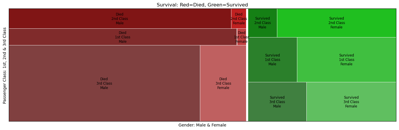
7
| # Mosaic Chart
plt.rc('figure', figsize=(17, 5))
mosaic(titanic_df, ['Survival', 'Class', 'Gender'], axes_label=False, title='Survival: Red=Died, Green=Survived')
plt.xlabel('Gender: Male & Female')
plt.ylabel('Passenger Class: 1st, 2nd & 3rd Class')
plt.show()
|
1
2
3
4
5
6
7
8
9
10
11
12
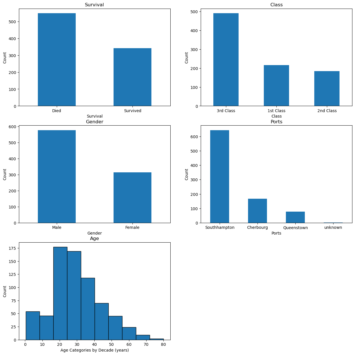
13
| cols = ['Survival', 'Class', 'Gender', 'Ports']
fig, axes = plt.subplots(nrows=3, ncols=2, figsize=(15, 15))
axes = axes.flat
for col, ax in zip(cols, axes):
titanic_df[col].value_counts().plot(kind='bar', title=col, ax=ax, rot=0, ylabel='Count')
titanic_df['Age'].plot(kind='hist', ax=axes[4], ylabel='Count', xlabel='Age Categories by Decade (years)', ec='k', title='Age')
fig.delaxes(axes[5])
|
Age
1
2
3
| # Passangers with no age
ageisnull = titanic_df[titanic_df['Age'].isnull()]
ageisnull.head()
|
| Survived | Pclass | Sex | Age | Parch | Fare | Embarked | Sex_Numeric | Survival | Class | Gender | Ports |
|---|
| 5 | 0 | 3 | male | NaN | 0 | 8.4583 | Q | 1 | Died | 3rd Class | Male | Queenstown |
|---|
| 17 | 1 | 2 | male | NaN | 0 | 13.0000 | S | 1 | Survived | 2nd Class | Male | Southhampton |
|---|
| 19 | 1 | 3 | female | NaN | 0 | 7.2250 | C | 0 | Survived | 3rd Class | Female | Cherbourg |
|---|
| 26 | 0 | 3 | male | NaN | 0 | 7.2250 | C | 1 | Died | 3rd Class | Male | Cherbourg |
|---|
| 28 | 1 | 3 | female | NaN | 0 | 7.8792 | Q | 0 | Survived | 3rd Class | Female | Queenstown |
|---|
1
| print('Total passengers with no age: ', len(ageisnull))
|
1
| Total passengers with no age: 177
|
In the Dataset Exploration section, it was determined there were only 714 of 891 valid age related records. We can see there are 177 NaN entries for Age.
1
2
| # Mean age
titanic_df['Age'].mean()
|
1
2
| # Mean age by Sex
(titanic_df.groupby(['Gender']))['Age'].mean()
|
1
2
3
4
| Gender
Female 27.915709
Male 30.726645
Name: Age, dtype: float64
|
1
2
| # Mean age by Pclass and Sex
(titanic_df.groupby(['Class', 'Gender']))['Age'].mean()
|
1
2
3
4
5
6
7
8
| Class Gender
1st Class Female 34.611765
Male 41.281386
2nd Class Female 28.722973
Male 30.740707
3rd Class Female 21.750000
Male 26.507589
Name: Age, dtype: float64
|
1
2
| # Mean age by Pclass, Survived and Sex
(titanic_df.groupby(['Class', 'Survival', 'Gender']))['Age'].mean()
|
1
2
3
4
5
6
7
8
9
10
11
12
13
14
| Class Survival Gender
1st Class Died Female 25.666667
Male 44.581967
Survived Female 34.939024
Male 36.248000
2nd Class Died Female 36.000000
Male 33.369048
Survived Female 28.080882
Male 16.022000
3rd Class Died Female 23.818182
Male 27.255814
Survived Female 19.329787
Male 22.274211
Name: Age, dtype: float64
|
1
2
| # General statistics of Age by Class, Survival and Gender
(titanic_df.groupby(['Class', 'Survival', 'Gender']))['Age'].describe()
|
| | | count | mean | std | min | 25% | 50% | 75% | max |
|---|
| Class | Survival | Gender | | | | | | | | |
|---|
| 1st Class | Died | Female | 3.0 | 25.666667 | 24.006943 | 2.00 | 13.50 | 25.0 | 37.50 | 50.0 |
|---|
| Male | 61.0 | 44.581967 | 14.457749 | 18.00 | 33.00 | 45.5 | 56.00 | 71.0 |
|---|
| Survived | Female | 82.0 | 34.939024 | 13.223014 | 14.00 | 23.25 | 35.0 | 44.00 | 63.0 |
|---|
| Male | 40.0 | 36.248000 | 14.936744 | 0.92 | 27.00 | 36.0 | 48.00 | 80.0 |
|---|
| 2nd Class | Died | Female | 6.0 | 36.000000 | 12.915107 | 24.00 | 26.25 | 32.5 | 42.50 | 57.0 |
|---|
| Male | 84.0 | 33.369048 | 12.158125 | 16.00 | 24.75 | 30.5 | 39.00 | 70.0 |
|---|
| Survived | Female | 68.0 | 28.080882 | 12.764693 | 2.00 | 21.75 | 28.0 | 35.25 | 55.0 |
|---|
| Male | 15.0 | 16.022000 | 19.547122 | 0.67 | 1.00 | 3.0 | 31.50 | 62.0 |
|---|
| 3rd Class | Died | Female | 55.0 | 23.818182 | 12.833465 | 2.00 | 15.25 | 22.0 | 31.00 | 48.0 |
|---|
| Male | 215.0 | 27.255814 | 12.135707 | 1.00 | 20.00 | 25.0 | 34.00 | 74.0 |
|---|
| Survived | Female | 47.0 | 19.329787 | 12.303246 | 0.75 | 13.50 | 19.0 | 26.50 | 63.0 |
|---|
| Male | 38.0 | 22.274211 | 11.555786 | 0.42 | 16.50 | 25.0 | 29.75 | 45.0 |
|---|
1
2
3
4
5
6
7
| # Survival count by Sex, Pclass and Age < 20
sex = titanic_df['Gender']
survived = titanic_df['Survival']
pclass = titanic_df['Class']
age_youth = titanic_df['Age'] < 20
pd.crosstab([sex, pclass, age_youth], survived)
|
| | Survival | Died | Survived |
|---|
| Gender | Class | Age | | |
|---|
| Female | 1st Class | False | 2 | 78 |
|---|
| True | 1 | 13 |
|---|
| 2nd Class | False | 6 | 54 |
|---|
| True | 0 | 16 |
|---|
| 3rd Class | False | 51 | 48 |
|---|
| True | 21 | 24 |
|---|
| Male | 1st Class | False | 74 | 41 |
|---|
| True | 3 | 4 |
|---|
| 2nd Class | False | 82 | 7 |
|---|
| True | 9 | 10 |
|---|
| 3rd Class | False | 249 | 35 |
|---|
| True | 51 | 12 |
|---|
A decision is required to determine the best method of dealing with NaN values.
- The NaN values can be ignored
- NaN can be filled in with a value, typically a mean
- Comparing the counts for various groups leads to the conclusion, simply using the overall mean will heavily weigh one specific age and skew any age dependant results.
- For the remainder of this analytic process, the NaN values data will be replaced with a mean age based upon Pclass, Survived and Sex.
1
2
| # Maintain Age and create Age_Fill (populate missing ages)
titanic_df['Age_Fill'] = titanic_df['Age']
|
1
2
3
| titanic_df['Age_Fill'] = titanic_df['Age_Fill'] \
.groupby([titanic_df['Pclass'], titanic_df['Survived'], titanic_df['Sex']], observed=False) \
.transform(lambda x: x.fillna(x.mean())).to_frame()
|
Create a new category called Age_Fill and fill NaN with an age based upon the mean of Pclass, Survived and Sex.
1
2
3
| # Example of Age_Fill - #5, 17 & 19
print(titanic_df['Age'].head(20))
print(titanic_df['Age_Fill'].head(20))
|
1
2
3
4
5
6
7
8
9
10
11
12
13
14
15
16
17
18
19
20
21
22
23
24
25
26
27
28
29
30
31
32
33
34
35
36
37
38
39
40
41
42
| 0 22.0
1 38.0
2 26.0
3 35.0
4 35.0
5 NaN
6 54.0
7 2.0
8 27.0
9 14.0
10 4.0
11 58.0
12 20.0
13 39.0
14 14.0
15 55.0
16 2.0
17 NaN
18 31.0
19 NaN
Name: Age, dtype: float64
0 22.000000
1 38.000000
2 26.000000
3 35.000000
4 35.000000
5 27.255814
6 54.000000
7 2.000000
8 27.000000
9 14.000000
10 4.000000
11 58.000000
12 20.000000
13 39.000000
14 14.000000
15 55.000000
16 2.000000
17 16.022000
18 31.000000
19 19.329787
Name: Age_Fill, dtype: float64
|
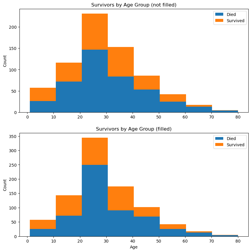
Age Histogram Comparison
1
2
3
4
5
6
7
8
9
10
11
12
13
14
15
16
17
18
19
20
21
22
23
24
25
26
27
28
29
30
31
| # Setup a figue of plots
df1 = titanic_df[titanic_df['Survived'] == 0]['Age']
df2 = titanic_df[titanic_df['Survived'] == 1]['Age']
df3 = titanic_df[titanic_df['Survived'] == 0]['Age_Fill']
df4 = titanic_df[titanic_df['Survived'] == 1]['Age_Fill']
max_age = max(titanic_df['Age_Fill'])
fig, (ax1, ax2) = plt.subplots(nrows=2, ncols=1, figsize=(10, 10))
ax1.hist([df1, df2],
bins=8,
range=(1, max_age),
stacked=True)
ax1.legend(('Died', 'Survived'), loc='best')
ax1.set_title('Survivors by Age Group (not filled)')
ax1.set_ylabel('Count')
ax2.hist([df3, df4],
bins=8,
range=(1, max_age),
stacked=True)
ax2.legend(('Died', 'Survived'), loc='best')
ax2.set_title('Survivors by Age Group (filled)')
ax2.set_xlabel('Age')
ax2.set_ylabel('Count')
plt.show()
|
1
2
| # Maximum age
titanic_df['Age'].max()
|
1
2
3
4
5
6
7
8
| # Create a new column that has all ages by bin category: 0-10:10, 10-20:20, 20-30:30, 30-40:40
# 40-50:50, 50-60:60, 60-70:70, 70-80:80
bins = [0, 10, 20, 30, 40, 50, 60, 70, 80]
group_names = [10, 20, 30, 40, 50, 60, 70, 80]
titanic_df['Age_Categories'] = pd.cut(titanic_df['Age_Fill'], bins, labels=group_names)
titanic_df[['Age', 'Age_Fill', 'Age_Categories']].head()
|
| Age | Age_Fill | Age_Categories |
|---|
| 0 | 22.0 | 22.0 | 30 |
|---|
| 1 | 38.0 | 38.0 | 40 |
|---|
| 2 | 26.0 | 26.0 | 30 |
|---|
| 3 | 35.0 | 35.0 | 40 |
|---|
| 4 | 35.0 | 35.0 | 40 |
|---|
1
| titanic_df['Age_Categories'] = pd.to_numeric(titanic_df['Age_Categories'])
|
An Age_Categories column has been inserted into the dataframe to simplify certain visualizations and calculations, as there are to many individual ages to easily draw conclusions or see patterns.
1
2
| # Survival Count by Age_Categories
titanic_df.groupby('Survival')[['Age_Categories']].count()
|
| Age_Categories |
|---|
| Survival | |
|---|
| Died | 549 |
|---|
| Survived | 342 |
|---|
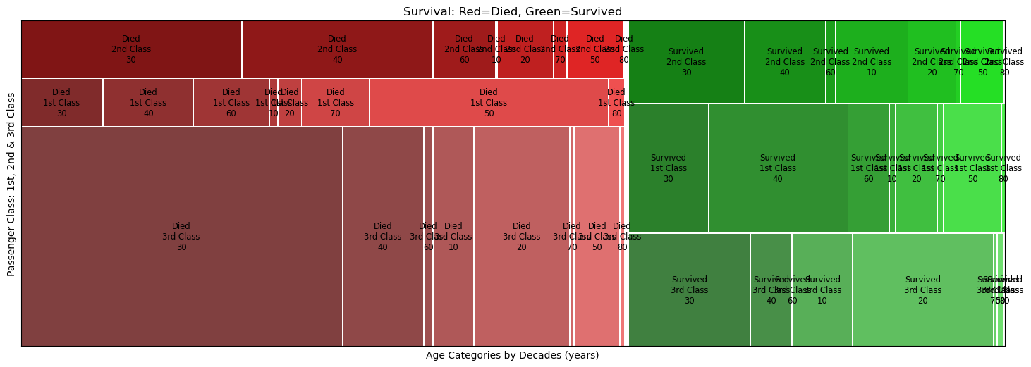
Age Mosaic
1
2
3
4
5
6
7
| # Mosaic Plot
plt.rc('figure', figsize=(18, 6)) # figure size
mosaic(titanic_df,['Survival', 'Class', 'Age_Categories'], axes_label=False, title='Survival: Red=Died, Green=Survived')
plt.xlabel('Age Categories by Decades (years)')
plt.ylabel('Passenger Class: 1st, 2nd & 3rd Class')
plt.show()
|
1
2
3
4
5
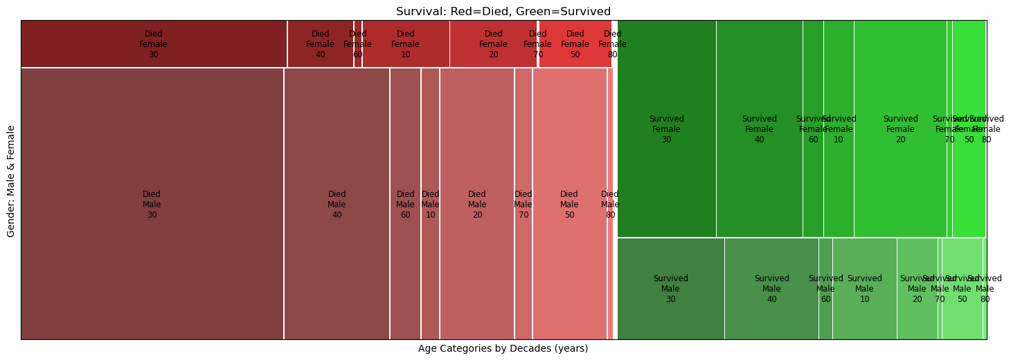
| # Mosaic Plot
mosaic(titanic_df,['Survival', 'Gender', 'Age_Categories'], axes_label=False, title='Survival: Red=Died, Green=Survived')
plt.xlabel('Age Categories by Decades (years)')
plt.ylabel('Gender: Male & Female')
plt.show()
|
Pclass
1
2
3
| # Survival count by Pclass
pclass_ct = titanic_df.groupby('Class')['Survival'].value_counts().unstack()
pclass_ct
|
| Survival | Died | Survived |
|---|
| Class | | |
|---|
| 1st Class | 80 | 136 |
|---|
| 2nd Class | 97 | 87 |
|---|
| 3rd Class | 372 | 119 |
|---|
1
2
| # Survival Rate
titanic_df.groupby('Class')['Survival'].value_counts(normalize = True).unstack()
|
| Survival | Died | Survived |
|---|
| Class | | |
|---|
| 1st Class | 0.370370 | 0.629630 |
|---|
| 2nd Class | 0.527174 | 0.472826 |
|---|
| 3rd Class | 0.757637 | 0.242363 |
|---|
1
2
3
4
5
6
7
8
9
10
| # Setup a figure of plots
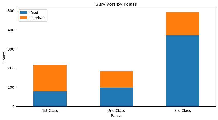
pclass_ct.plot(kind='bar', stacked=True, figsize=(10, 5))
plt.legend(('Died', 'Survived'), loc='best')
plt.title('Survivors by Pclass')
plt.xlabel('Pclass')
plt.ylabel('Count')
plt.xticks(rotation=0)
plt.show()
|
Pclass is not a strong indicator for surviving, however 3rd Class is a stong indicator for dying.
Sex
1
2
3
| # Survival count by sex
sex_ct = titanic_df.groupby('Gender')['Survival'].value_counts().unstack()
sex_ct
|
| Survival | Died | Survived |
|---|
| Gender | | |
|---|
| Female | 81 | 233 |
|---|
| Male | 468 | 109 |
|---|
1
2
| # Survival rate by sex
titanic_df.groupby('Gender')['Survival'].value_counts(normalize = True).unstack()
|
| Survival | Died | Survived |
|---|
| Gender | | |
|---|
| Female | 0.257962 | 0.742038 |
|---|
| Male | 0.811092 | 0.188908 |
|---|
1
2
3
4
5
6
7
8
9
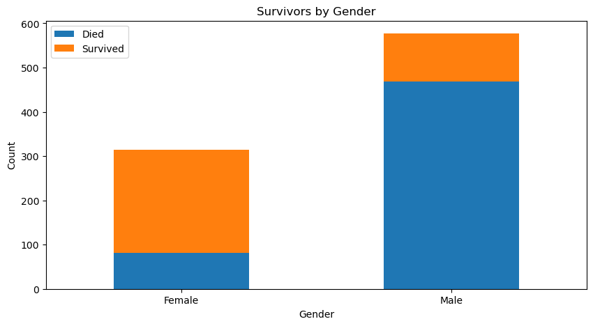
| sex_ct.plot(kind='bar', stacked=True, figsize=(10, 5))
plt.legend(('Died', 'Survived'), loc='best')
plt.title('Survivors by Gender')
plt.xlabel('Gender')
plt.ylabel('Count')
plt.xticks(rotation=0)
plt.show()
|
Gender is a strong indicator for survivability, with a significant portion of females (74%) surviving and males 81% dying.
Embarked
1
2
3
4
| # Survival count by Embarked
embarked_ct = titanic_df.groupby('Ports')['Survival'].value_counts().unstack()
embarked_ct
|
| Survival | Died | Survived |
|---|
| Ports | | |
|---|
| Cherbourg | 75.0 | 93.0 |
|---|
| Queenstown | 47.0 | 30.0 |
|---|
| Southhampton | 427.0 | 217.0 |
|---|
| unknown | NaN | 2.0 |
|---|
1
2
| # Survival rate by embarked
titanic_df.groupby('Ports')['Survival'].value_counts(normalize = True).unstack()
|
| Survival | Died | Survived |
|---|
| Ports | | |
|---|
| Cherbourg | 0.446429 | 0.553571 |
|---|
| Queenstown | 0.610390 | 0.389610 |
|---|
| Southhampton | 0.663043 | 0.336957 |
|---|
| unknown | NaN | 1.000000 |
|---|
1
2
3
4
5
6
7
8
9
10
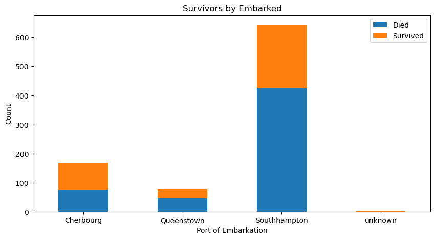
| plt.rc('figure', figsize=(10, 5))
embarked_ct.plot(kind='bar', stacked=True, figsize=(10, 5), rot=0)
plt.legend(('Died', 'Survived'), loc='best')
plt.title('Survivors by Embarked')
plt.xlabel('Port of Embarkation')
plt.ylabel('Count')
plt.show()
|
Statistics
1
2
3
4
5
6
7
| # Survival count by Sex, Embarked_Numeric, Pclass and Age Category
embarked = titanic_df['Ports']
sex = titanic_df['Gender']
survived = titanic_df['Survival']
pclass = titanic_df['Class']
age_cat = titanic_df['Age_Categories']
pd.crosstab([sex, embarked, pclass], [survived, age_cat])
|
| | Survival | Died | Survived |
|---|
| | Age_Categories | 10 | 20 | 30 | 40 | 50 | 60 | 70 | 80 | 10 | 20 | 30 | 40 | 50 | 60 | 70 | 80 |
|---|
| Gender | Ports | Class | | | | | | | | | | | | | | | | |
|---|
| Female | Cherbourg | 1st Class | 0 | 0 | 0 | 0 | 1 | 0 | 0 | 0 | 0 | 5 | 10 | 14 | 7 | 6 | 0 | 0 |
|---|
| 2nd Class | 0 | 0 | 0 | 0 | 0 | 0 | 0 | 0 | 1 | 2 | 4 | 0 | 0 | 0 | 0 | 0 |
|---|
| 3rd Class | 1 | 3 | 3 | 0 | 1 | 0 | 0 | 0 | 5 | 8 | 2 | 0 | 0 | 0 | 0 | 0 |
|---|
| Queenstown | 1st Class | 0 | 0 | 0 | 0 | 0 | 0 | 0 | 0 | 0 | 0 | 0 | 1 | 0 | 0 | 0 | 0 |
|---|
| 2nd Class | 0 | 0 | 0 | 0 | 0 | 0 | 0 | 0 | 0 | 0 | 2 | 0 | 0 | 0 | 0 | 0 |
|---|
| 3rd Class | 0 | 1 | 5 | 3 | 0 | 0 | 0 | 0 | 0 | 23 | 1 | 0 | 0 | 0 | 0 | 0 |
|---|
| Southhampton | 1st Class | 1 | 0 | 1 | 0 | 0 | 0 | 0 | 0 | 0 | 8 | 10 | 17 | 5 | 5 | 1 | 0 |
|---|
| 2nd Class | 0 | 0 | 3 | 1 | 1 | 1 | 0 | 0 | 7 | 6 | 21 | 16 | 9 | 2 | 0 | 0 |
|---|
| 3rd Class | 10 | 8 | 25 | 5 | 7 | 0 | 0 | 0 | 6 | 7 | 13 | 6 | 0 | 0 | 1 | 0 |
|---|
| unknown | 1st Class | 0 | 0 | 0 | 0 | 0 | 0 | 0 | 0 | 0 | 0 | 0 | 1 | 0 | 0 | 1 | 0 |
|---|
| Male | Cherbourg | 1st Class | 0 | 1 | 6 | 3 | 8 | 4 | 1 | 2 | 0 | 1 | 5 | 6 | 3 | 2 | 0 | 0 |
|---|
| 2nd Class | 0 | 0 | 4 | 4 | 0 | 0 | 0 | 0 | 1 | 1 | 0 | 0 | 0 | 0 | 0 | 0 |
|---|
| 3rd Class | 0 | 4 | 23 | 5 | 1 | 0 | 0 | 0 | 1 | 3 | 6 | 0 | 0 | 0 | 0 | 0 |
|---|
| Queenstown | 1st Class | 0 | 0 | 0 | 0 | 1 | 0 | 0 | 0 | 0 | 0 | 0 | 0 | 0 | 0 | 0 | 0 |
|---|
| 2nd Class | 0 | 0 | 0 | 0 | 0 | 1 | 0 | 0 | 0 | 0 | 0 | 0 | 0 | 0 | 0 | 0 |
|---|
| 3rd Class | 4 | 1 | 25 | 3 | 1 | 0 | 1 | 1 | 0 | 0 | 3 | 0 | 0 | 0 | 0 | 0 |
|---|
| Southhampton | 1st Class | 0 | 2 | 4 | 9 | 22 | 6 | 8 | 0 | 2 | 1 | 4 | 12 | 6 | 2 | 0 | 1 |
|---|
| 2nd Class | 0 | 9 | 29 | 26 | 8 | 8 | 2 | 0 | 8 | 2 | 0 | 3 | 1 | 0 | 1 | 0 |
|---|
| 3rd Class | 10 | 42 | 120 | 34 | 18 | 5 | 1 | 1 | 7 | 4 | 14 | 7 | 2 | 0 | 0 | 0 |
|---|
OLS Regression Models
1
2
3
| # OLS modeling for Survived and Gender
result_1 = sm.ols(formula='Survived ~ Gender', data=titanic_df).fit()
result_1.summary()
|
OLS Regression Results| Dep. Variable: | Survived | R-squared: | 0.295 |
|---|
| Model: | OLS | Adj. R-squared: | 0.294 |
|---|
| Method: | Least Squares | F-statistic: | 372.4 |
|---|
| Date: | Sat, 13 Apr 2024 | Prob (F-statistic): | 1.41e-69 |
|---|
| Time: | 11:21:22 | Log-Likelihood: | -466.09 |
|---|
| No. Observations: | 891 | AIC: | 936.2 |
|---|
| Df Residuals: | 889 | BIC: | 945.8 |
|---|
| Df Model: | 1 | | |
|---|
| Covariance Type: | nonrobust | | |
|---|
| coef | std err | t | P>|t| | [0.025 | 0.975] |
|---|
| Intercept | 0.7420 | 0.023 | 32.171 | 0.000 | 0.697 | 0.787 |
|---|
| Gender[T.Male] | -0.5531 | 0.029 | -19.298 | 0.000 | -0.609 | -0.497 |
|---|
| Omnibus: | 25.424 | Durbin-Watson: | 1.959 |
|---|
| Prob(Omnibus): | 0.000 | Jarque-Bera (JB): | 27.169 |
|---|
| Skew: | 0.427 | Prob(JB): | 1.26e-06 |
|---|
| Kurtosis: | 2.963 | Cond. No. | 3.13 |
|---|
Notes:
[1] Standard Errors assume that the covariance matrix of the errors is correctly specified.
1
2
3
| # OLS modeling for Survived and Class
result_2 = sm.ols(formula='Survived ~ Class', data=titanic_df).fit()
result_2.summary()
|
OLS Regression Results| Dep. Variable: | Survived | R-squared: | 0.115 |
|---|
| Model: | OLS | Adj. R-squared: | 0.113 |
|---|
| Method: | Least Squares | F-statistic: | 57.96 |
|---|
| Date: | Sat, 13 Apr 2024 | Prob (F-statistic): | 2.18e-24 |
|---|
| Time: | 11:21:22 | Log-Likelihood: | -567.30 |
|---|
| No. Observations: | 891 | AIC: | 1141. |
|---|
| Df Residuals: | 888 | BIC: | 1155. |
|---|
| Df Model: | 2 | | |
|---|
| Covariance Type: | nonrobust | | |
|---|
| coef | std err | t | P>|t| | [0.025 | 0.975] |
|---|
| Intercept | 0.6296 | 0.031 | 20.198 | 0.000 | 0.568 | 0.691 |
|---|
| Class[T.2nd Class] | -0.1568 | 0.046 | -3.412 | 0.001 | -0.247 | -0.067 |
|---|
| Class[T.3rd Class] | -0.3873 | 0.037 | -10.353 | 0.000 | -0.461 | -0.314 |
|---|
| Omnibus: | 1364.423 | Durbin-Watson: | 1.957 |
|---|
| Prob(Omnibus): | 0.000 | Jarque-Bera (JB): | 86.840 |
|---|
| Skew: | 0.421 | Prob(JB): | 1.39e-19 |
|---|
| Kurtosis: | 1.723 | Cond. No. | 4.56 |
|---|
Notes:
[1] Standard Errors assume that the covariance matrix of the errors is correctly specified.
1
2
3
| # OLS modeling for Survived and Ports
result_3 = sm.ols(formula='Survived ~ Ports', data=titanic_df).fit()
result_3.summary()
|
OLS Regression Results| Dep. Variable: | Survived | R-squared: | 0.033 |
|---|
| Model: | OLS | Adj. R-squared: | 0.030 |
|---|
| Method: | Least Squares | F-statistic: | 10.18 |
|---|
| Date: | Sat, 13 Apr 2024 | Prob (F-statistic): | 1.34e-06 |
|---|
| Time: | 11:21:23 | Log-Likelihood: | -606.87 |
|---|
| No. Observations: | 891 | AIC: | 1222. |
|---|
| Df Residuals: | 887 | BIC: | 1241. |
|---|
| Df Model: | 3 | | |
|---|
| Covariance Type: | nonrobust | | |
|---|
| coef | std err | t | P>|t| | [0.025 | 0.975] |
|---|
| Intercept | 0.5536 | 0.037 | 14.972 | 0.000 | 0.481 | 0.626 |
|---|
| Ports[T.Queenstown] | -0.1640 | 0.066 | -2.486 | 0.013 | -0.293 | -0.035 |
|---|
| Ports[T.Southhampton] | -0.2166 | 0.042 | -5.218 | 0.000 | -0.298 | -0.135 |
|---|
| Ports[T.unknown] | 0.4464 | 0.341 | 1.310 | 0.191 | -0.223 | 1.115 |
|---|
| Omnibus: | 4800.327 | Durbin-Watson: | 1.981 |
|---|
| Prob(Omnibus): | 0.000 | Jarque-Bera (JB): | 133.483 |
|---|
| Skew: | 0.478 | Prob(JB): | 1.03e-29 |
|---|
| Kurtosis: | 1.362 | Cond. No. | 26.9 |
|---|
Notes:
[1] Standard Errors assume that the covariance matrix of the errors is correctly specified.
1
2
3
| # OLS modeling for Survived and Age_Fill
result_4 = sm.ols(formula='Survived ~ Age_Fill', data=titanic_df).fit()
result_4.summary()
|
OLS Regression Results| Dep. Variable: | Survived | R-squared: | 0.009 |
|---|
| Model: | OLS | Adj. R-squared: | 0.008 |
|---|
| Method: | Least Squares | F-statistic: | 7.998 |
|---|
| Date: | Sat, 13 Apr 2024 | Prob (F-statistic): | 0.00479 |
|---|
| Time: | 11:21:23 | Log-Likelihood: | -617.97 |
|---|
| No. Observations: | 891 | AIC: | 1240. |
|---|
| Df Residuals: | 889 | BIC: | 1250. |
|---|
| Df Model: | 1 | | |
|---|
| Covariance Type: | nonrobust | | |
|---|
| coef | std err | t | P>|t| | [0.025 | 0.975] |
|---|
| Intercept | 0.4847 | 0.039 | 12.372 | 0.000 | 0.408 | 0.562 |
|---|
| Age_Fill | -0.0034 | 0.001 | -2.828 | 0.005 | -0.006 | -0.001 |
|---|
| Omnibus: | 4214.198 | Durbin-Watson: | 1.956 |
|---|
| Prob(Omnibus): | 0.000 | Jarque-Bera (JB): | 145.594 |
|---|
| Skew: | 0.474 | Prob(JB): | 2.42e-32 |
|---|
| Kurtosis: | 1.262 | Cond. No. | 77.8 |
|---|
Notes:
[1] Standard Errors assume that the covariance matrix of the errors is correctly specified.
1
2
3
| # OLS modeling for Survived and Gender + Class + Age_Fill + Ports
result_5 = sm.ols(formula='Survived ~ Gender + Class + Age_Fill + Ports', data=titanic_df).fit()
result_5.summary()
|
OLS Regression Results| Dep. Variable: | Survived | R-squared: | 0.399 |
|---|
| Model: | OLS | Adj. R-squared: | 0.394 |
|---|
| Method: | Least Squares | F-statistic: | 83.64 |
|---|
| Date: | Sat, 13 Apr 2024 | Prob (F-statistic): | 3.69e-93 |
|---|
| Time: | 11:21:23 | Log-Likelihood: | -395.35 |
|---|
| No. Observations: | 891 | AIC: | 806.7 |
|---|
| Df Residuals: | 883 | BIC: | 845.0 |
|---|
| Df Model: | 7 | | |
|---|
| Covariance Type: | nonrobust | | |
|---|
| coef | std err | t | P>|t| | [0.025 | 0.975] |
|---|
| Intercept | 1.1928 | 0.051 | 23.260 | 0.000 | 1.092 | 1.293 |
|---|
| Gender[T.Male] | -0.4758 | 0.028 | -17.243 | 0.000 | -0.530 | -0.422 |
|---|
| Class[T.2nd Class] | -0.1777 | 0.041 | -4.366 | 0.000 | -0.258 | -0.098 |
|---|
| Class[T.3rd Class] | -0.3939 | 0.036 | -10.818 | 0.000 | -0.465 | -0.322 |
|---|
| Ports[T.Queenstown] | -0.0104 | 0.055 | -0.191 | 0.849 | -0.118 | 0.097 |
|---|
| Ports[T.Southhampton] | -0.0777 | 0.034 | -2.254 | 0.024 | -0.145 | -0.010 |
|---|
| Ports[T.unknown] | 0.1316 | 0.271 | 0.486 | 0.627 | -0.400 | 0.663 |
|---|
| Age_Fill | -0.0065 | 0.001 | -6.091 | 0.000 | -0.009 | -0.004 |
|---|
| Omnibus: | 36.566 | Durbin-Watson: | 1.922 |
|---|
| Prob(Omnibus): | 0.000 | Jarque-Bera (JB): | 40.062 |
|---|
| Skew: | 0.514 | Prob(JB): | 2.00e-09 |
|---|
| Kurtosis: | 3.156 | Cond. No. | 689. |
|---|
Notes:
[1] Standard Errors assume that the covariance matrix of the errors is correctly specified.
1
2
3
| # OLS modeling for Survived and Gender + Class + Age_Fill
result_6 = sm.ols(formula='Survived ~ Gender + Class + Age_Fill', data=titanic_df).fit()
result_6.summary()
|
OLS Regression Results| Dep. Variable: | Survived | R-squared: | 0.394 |
|---|
| Model: | OLS | Adj. R-squared: | 0.391 |
|---|
| Method: | Least Squares | F-statistic: | 144.0 |
|---|
| Date: | Sat, 13 Apr 2024 | Prob (F-statistic): | 7.26e-95 |
|---|
| Time: | 11:21:23 | Log-Likelihood: | -398.78 |
|---|
| No. Observations: | 891 | AIC: | 807.6 |
|---|
| Df Residuals: | 886 | BIC: | 831.5 |
|---|
| Df Model: | 4 | | |
|---|
| Covariance Type: | nonrobust | | |
|---|
| coef | std err | t | P>|t| | [0.025 | 0.975] |
|---|
| Intercept | 1.1573 | 0.048 | 23.887 | 0.000 | 1.062 | 1.252 |
|---|
| Gender[T.Male] | -0.4845 | 0.027 | -17.708 | 0.000 | -0.538 | -0.431 |
|---|
| Class[T.2nd Class] | -0.2033 | 0.039 | -5.184 | 0.000 | -0.280 | -0.126 |
|---|
| Class[T.3rd Class] | -0.4069 | 0.035 | -11.747 | 0.000 | -0.475 | -0.339 |
|---|
| Age_Fill | -0.0066 | 0.001 | -6.200 | 0.000 | -0.009 | -0.005 |
|---|
| Omnibus: | 34.024 | Durbin-Watson: | 1.911 |
|---|
| Prob(Omnibus): | 0.000 | Jarque-Bera (JB): | 36.990 |
|---|
| Skew: | 0.494 | Prob(JB): | 9.28e-09 |
|---|
| Kurtosis: | 3.143 | Cond. No. | 157. |
|---|
Notes:
[1] Standard Errors assume that the covariance matrix of the errors is correctly specified.
1
2
3
4
5
6
7
8
9
10
11
12
13
14
15
16
| # Dataframe for statistical data
comp_index_4 = 'Gender + Class + Age_Fill + Ports'
comp_index_3 = 'Gender + Class + Age_Fill'
statistics_df = pd.DataFrame(
data=[[result_1.rsquared_adj, np.sqrt(result_1.rsquared_adj)],
[result_2.rsquared_adj, np.sqrt(result_2.rsquared_adj)],
[result_3.rsquared_adj, np.sqrt(result_3.rsquared_adj)],
[result_4.rsquared_adj, np.sqrt(result_4.rsquared_adj)],
[result_5.rsquared_adj, np.sqrt(result_5.rsquared_adj)],
[result_6.rsquared_adj, np.sqrt(result_6.rsquared_adj)]],
index=['Gender', 'Class', 'Ports', 'Age_Fill', comp_index_4, comp_index_3],
columns=['R-squared', 'Correlation to Survival']
)
statistics_df
|
| R-squared | Correlation to Survival |
|---|
| Gender | 0.294438 | 0.542621 |
|---|
| Class | 0.113484 | 0.336873 |
|---|
| Ports | 0.030031 | 0.173294 |
|---|
| Age_Fill | 0.007802 | 0.088329 |
|---|
| Gender + Class + Age_Fill + Ports | 0.393939 | 0.627645 |
|---|
| Gender + Class + Age_Fill | 0.391324 | 0.625559 |
|---|
Ordinary least squares (OLS) regression modeling has been used to determine which metric or combination of metrics provides the best prediction of survival. As can be determined by reviewing the coefficient of determination (R-squared), the individual models for Ports and Age_Fill indicate a large proportion of variance for survival. Gender and a combination of metrics are better models. The square root of R-squared equals the Pearson correlation coefficient of predicted to actual values; Gender is the single metric with the strongest correlation. However, the combination of metrics, Gender + Class + Age_Fill + Ports, shows the strongest correlation to survival for the model used.