Case Study - School Budgeting with Machine Learning in Python

Posted Jan 19, 2024 Updated Apr 27, 2024

By Trenton McKinney 111 min read

Introduction

GitHub Repository
Course: DataCamp: Case Study: School Budgeting with Machine Learning in Python - This notebook was created as a reproducible reference
If you find the content beneficial, consider a DataCamp Subscription

Course Description

Data science isn’t just for predicting ad-clicks-it’s also useful for social impact! This course is a case study from a machine learning competition on DrivenData. You’ll explore a problem related to school district budgeting. By building a model to automatically classify items in a school’s budget, it makes it easier and faster for schools to compare their spending with other schools. In this course, you’ll begin by building a baseline model that is a simple, first-pass approach. In particular, you’ll do some natural language processing to prepare the budgets for modeling. Next, you’ll have the opportunity to try your own techniques and see how they compare to participants from the competition. Finally, you’ll see how the winner was able to combine a number of expert techniques to build the most accurate model.

The case study discusses the use of several types of models for a school budgeting problem with machine learning in Python. The models used include:

Multi-class logistic regression: This is used as a starting point to quickly go from raw data to predictions. The model treats each label column independently and trains a logistic regression classifier for each label column separately.
Random Forest Classifier: This model is mentioned as a possible choice to use in a scikit-learn Pipeline for classification. It’s known for its performance and ease of use in classification tasks.
Naive Bayes Classifier: This is another type of model that could be used in a scikit-learn Pipeline. It is based on applying Bayes’ theorem with strong (naïve) independence assumptions between the features.
K-Nearest Neighbors (k-NN) Classifier: This model is listed as an alternative that could be experimented with in the pipeline. It classifies data based on the closest training examples in the feature space.
Ensemble methods: The document also alludes to the use of ensemble methods, which combine the predictions of multiple machine learning models to improve accuracy. Specifically, it mentions the winner of a competition using an ensemble of many models for classification.
Deep Convolutional Neural Network: It is indicated that the winner of a machine learning competition mentioned in the case study used a 500-layer deep convolutional neural network to master the budget data.

These models are typical in machine learning tasks that involve classification and pattern recognition. They were chosen for their effectiveness in dealing with the specific characteristics of the school budget data, such as its multi-class nature and the presence of both numerical and textual data.

Imports

DataCamp package versions vs. local versions:
- sklearn v0.20.4 vs. 1.3.2
- numpy v1.17.4 vs. 1.26.3
- pandas v0.24.2 vs. 2.2.1
- matplotlib v3.1.2 vs. 3.8.1

  
import pandas as pd
import matplotlib.pyplot as plt
import numpy as np
from typing import List, Union
import os

  
from sklearn.linear_model import LogisticRegression
from sklearn.multiclass import OneVsRestClassifier
from sklearn.feature_extraction.text import CountVectorizer, HashingVectorizer

from sklearn.pipeline import Pipeline
from sklearn.model_selection import train_test_split
from sklearn.impute import SimpleImputer

from sklearn.preprocessing import FunctionTransformer, MaxAbsScaler, PolynomialFeatures
from sklearn.pipeline import FeatureUnion

from sklearn.ensemble import RandomForestClassifier
from sklearn.feature_selection import chi2, SelectKBest
from sklearn.metrics import make_scorer

  
import sys
sys.path.append(r'D:\users\trenton\Dropbox\PythonProjects\DataCamp\functions')

from multilabel import multilabel_train_test_split
from score_sub import score_submission, _multi_multi_log_loss
from sparse_interactions import SparseInteractions

  
pd.set_option('display.max_columns', 700)
pd.set_option('display.max_rows', 400)
pd.set_option('display.min_rows', 10)
pd.set_option('display.expand_frame_repr', True)

Saving data from DataCamp to a local csv

  
# output the data to a format that can be copied and pasted into notepad++
# find all non and replace with np.nan
# copy all of lists and replace ... in data = np.array([...])
# print the columns names df.columns.tolist() and then create a variable in a notebook
# create a dataframe with df = pd.DataFrame(data=data, columns=columns)

# create the dataframe in the DataCamp console
df = pd.read_csv('TrainingData.csv')  # do not specify index_col=0

# print each row as a list with a comma at the end and then copy all of the lists into notepad++
for r in df.to_numpy():
    print(list(r), ',')

# print the column names and copy them
df.columns.tolist()

# in jupyterlab
data = np.array([...])  # replace ... with the cleaned lists from notepad++
columns = ...  # pasted from DataCamp console

df = pd.DataFrame(data=data, columns=columns)

df.to_csv('TrainingData.csv', index=False)

Exploring the Raw Data

In this chapter, you’ll be introduced to the problem you’ll be solving in this course. How do you accurately classify line-items in a school budget based on what that money is being used for? You will explore the raw text and numeric values in the dataset, both quantitatively and visually. And you’ll learn how to measure success when trying to predict class labels for each row of the dataset.

  
# set the current working directory if needed
cwd = os.getcwd()
if cwd != 'D:/Users/trenton/Dropbox/PythonProjects/DataCamp':
    os.chdir(r'D:\users\trenton\Dropbox\PythonProjects\DataCamp')

  
df = pd.read_csv('data/2024-01-19_school_budgeting_with_machine_learning_in_python/TrainingData.csv', index_col=0)

  
df.head()

	Function	Use	Sharing	Reporting	Student_Type	Position_Type	Object_Type	Pre_K	Operating_Status	Object_Description	Text_2	SubFund_Description	Job_Title_Description	Text_3	Text_4	Sub_Object_Description	Location_Description	FTE	Function_Description	Facility_or_Department	Position_Extra	Total	Program_Description	Fund_Description	Text_1
198	NO_LABEL	NO_LABEL	NO_LABEL	NO_LABEL	NO_LABEL	NO_LABEL	NO_LABEL	NO_LABEL	Non-Operating	Supplemental *	NaN	Operation and Maintenp.nance of Plant Services	NaN	NaN	NaN	Non-Certificated Salaries And Wages	NaN	NaN	Care and Upkeep of Building Services	NaN	NaN	-8291.86	NaN	Title I - Disadvantaged Children/Targeted Assi...	TITLE I CARRYOVER
209	Student Transportation	NO_LABEL	Shared Services	Non-School	NO_LABEL	NO_LABEL	Other Non-Compensation	NO_LABEL	PreK-12 Operating	REPAIR AND MAINTENANCE SERVICES	NaN	PUPIL TRANSPORTATION	NaN	NaN	NaN	NaN	ADMIN. SERVICES	NaN	STUDENT TRANSPORT SERVICE	NaN	NaN	618.29	PUPIL TRANSPORTATION	General Fund	NaN
750	Teacher Compensation	Instruction	School Reported	School	Unspecified	Teacher	Base Salary/Compensation	Non PreK	PreK-12 Operating	Personal Services - Teachers	NaN	NaN	TCHER 5TH GRADE	NaN	Regular Instruction	NaN	NaN	1.0	NaN	NaN	TEACHER	49768.82	Instruction - Regular	General Purpose School	NaN
931	NO_LABEL	NO_LABEL	NO_LABEL	NO_LABEL	NO_LABEL	NO_LABEL	NO_LABEL	NO_LABEL	Non-Operating	General Supplies	NaN	NaN	NaN	NaN	NaN	General Supplies	NaN	NaN	Instruction	Instruction And Curriculum	NaN	-1.02	"Title I, Part A Schoolwide Activities Related...	General Operating Fund	NaN
1524	NO_LABEL	NO_LABEL	NO_LABEL	NO_LABEL	NO_LABEL	NO_LABEL	NO_LABEL	NO_LABEL	Non-Operating	Supplies and Materials	NaN	Community Services	NaN	NaN	NaN	Supplies And Materials	NaN	NaN	Other Community Services *	NaN	NaN	2304.43	NaN	Title I - Disadvantaged Children/Targeted Assi...	TITLE I PI+HOMELESS

  
df.info()

<class 'pandas.core.frame.DataFrame'>
Index: 1560 entries, 198 to 101861
Data columns (total 25 columns):
 #   Column                  Non-Null Count  Dtype  
---  ------                  --------------  -----  
 Function                1560 non-null   object 
 Use                     1560 non-null   object 
 Sharing                 1560 non-null   object 
 Reporting               1560 non-null   object 
 Student_Type            1560 non-null   object 
 Position_Type           1560 non-null   object 
 Object_Type             1560 non-null   object 
 Pre_K                   1560 non-null   object 
 Operating_Status        1560 non-null   object 
 Object_Description      1461 non-null   object 
Text_2                  382 non-null    object 
SubFund_Description     1183 non-null   object 
Job_Title_Description   1131 non-null   object 
Text_3                  296 non-null    object 
Text_4                  193 non-null    object 
Sub_Object_Description  364 non-null    object 
Location_Description    874 non-null    object 
FTE                     449 non-null    float64
Function_Description    1340 non-null   object 
Facility_or_Department  252 non-null    object 
Position_Extra          1026 non-null   object 
Total                   1542 non-null   float64
Program_Description     1192 non-null   object 
Fund_Description        819 non-null    object 
Text_1                  1132 non-null   object 
dtypes: float64(2), object(23)
memory usage: 316.9+ KB

Introducing the challenge

Introducing the challenge: Hello DataCampers! How’s it going? Really glad you’ve decided to join us for this course. We have an exciting journey ahead of us through some real data and some incredibly useful tips and tricks from expert data scientists. I’m Peter Bull, a data scientist and a co-founder of DrivenData. Our mission is to bring the power of data science to social impact organizations. One of the ways we do that is by running online data science challenges for non-profits, NGOs, and social enterprises. In our challenges, a global community of data scientists–like you!–competes to solve a particular problem. We’ll work
- Learn from the expert who won DrivenData’s challenge
  - Natural language processing
  - Feature engineering
  - Efficency boosting hashing tricks
- Use data to have a social impact
Introducing the challenge: through one of these competitions as a case-study, and we’ll show you how the winner achieved the best score. In the course, we’ll do some natural language processing, some feature engineering, and boost our computational efficiency. In addition to these pro-tips, we’ll look at one of the ways in which we can use data to have a social impact.
- Budgets for schools are huge, complex, and not standardized
  - Hundreds of hours each year are spent manually labelling
- Goal: Build a machine learning algorithm that can automate the process
- Budget data
  - Line-item: “Algebra books for 8th grade students”
  - Labels: “Textbooks”, “Math”, “Middle School”
- This is a supervised learning problem
Introducing the challenge: School budgets in the United States are incredibly complex, and there are no standards for reporting how money is spent. Schools want to be able to measure their performance–for example, are we spending more on textbooks than our neighboring schools, and is that investment worthwhile? However to do this comparison takes hundreds of hours each year in which analysts hand-categorize each line-item. Our goal is to build a machine learning algorithm that can automate that process. For each line item, we have some text fields that tell us about the expense–for example, a line might say something like “Algebra books for 8th grade students”. We also have the amount of the expense in dollars. This line item then has a set of labels attached to it. For example, this one might have labels like “Textbooks,” “Math,” and “Middle School.” These labels are our target variable. This is a supervised learning problem where we want to use correctly labeled data to build an algorithm that can suggest labels for unlabeled lines. This is in contrast to an unsupervised learning problem where we don’t have labels, and we are using an algorithm to automatically which line-items might go together. For this problem,
Over 100 target variables!: we have over 100 unique target variables that could be attached to a single line item. Because we want to predict a category for each line item, this is a classification problem. This is as opposed to a regression problem where we want to predict a numeric value for a line item–for example, predicting house prices. Here are some of the actual categories that we need to determine: Is this expense for
Over 100 target variables!: pre-kindergarten education (which is important because it has different funding sources)? Or, is there a particular
Over 100 target variables!: Student_Type that this expense supports? Overall, there are 9 columns with many different possible categories in each column.
- This is a classification problem
  - Pre_K:
- NO_LABEL
- Non PreK
- PreK - Sharing:
- Leadership & Management
- NO_LABEL
- School Reported - Reporting:
- NO_LABEL
- Non-School
- School - Student_Type:
- Alternative
- At Risk
How we can help: If you talk to the people who actually do this work, it is impossible for a human to label these line items with 100% accuracy. To take this into account, we don’t want our algorithm to just say “This line is for textbooks.” We want it to say: “It’s most likely this line is for textbooks, and I’m 60% sure that it is. If it’s not textbooks, I’m 30% sure it’s ‘office supplies.’” By making these suggestions, analysts can prioritize their time. This is called a human-in-the-loop machine learning system.
How we can help: We will predict a probability between 0 (the algorithm thinks this label is very unlikely for this line item) and 1 (the algorithm thinks this label is very likely). We’ll take a quick break to review and then come back to talk about how to load the data.
- Predictions will be probabilites for each label
Let’s practice!: We’ll take a quick break to review and then come back to talk about how to load the data.

What category of problem is this?

You’re no novice to data science, but let’s make sure we agree on the basics.

As Peter from DrivenData explained in the video, you’re going to be working with school district budget data. This data can be classified in many ways according to certain labels, e.g. Function: Career & Academic Counseling, or Position_Type: Librarian.

Your goal is to develop a model that predicts the probability for each possible label by relying on some correctly labeled examples.

What type of machine learning problem is this?

Answer the question

~~Reinforcement Learning, because the model is learning from the data through a system of rewards and punishments.~~
~~Unsupervised Learning, because the model doesn’t output labels with certainty.~~
~~Unsupervised Learning, because not all data is correctly classified to begin with.~~
Supervised Learning, because the model will be trained using labeled examples. - Using correctly labeled budget line items to train means this is a supervised learning problem.

What is the goal of the algorithm?

As you know from previous courses, there are different types of supervised machine learning problems. In this exercise you will tell us what type of supervised machine learning problem this is, and why you think so.

Remember, your goal is to correctly label budget line items by training a supervised model to predict the probability of each possible label, taking most probable label as the correct label.

Answer the question

~~Regression, because the model will output probabilities.~~
Classification, because predicted probabilities will be used to select a label class. - Specifically, we have ourselves a multi-class-multi-label classification problem (quite a mouthful!), because there are 9 broad categories that each take on many possible sub-label instances.
~~Regression, because probabilities take a continuous value between 0 and 1.~~
~~Classification, because the model will output probabilities.~~

Exploring the data

Exploring the data: We left off the last video by showing that we’d be predicting probabilities for each budget line item. Let’s be clear what this looks like in practice.
A column for each possible value: or example, we’ll say we are predicting the hair type and eye color of people. We have the categories “curly,” “straight,” and “wavy” for hair and “brown” and “blue” for eyes. If we are predicting probabilities, we need a value for each possible value in each column. In this case, the target would have the columns for each hair type and for each eye color. Later in the course, we’ll talk more about how to perform this transformation. We’ll begin by loading our data.
Load and preview the data: As an example, in this video we’ll work with a small sample dataset. For the exercises, you’ll be loading the actual school budget dataset. You’ve seen pandas functions for loading data before, and in this case we’ll be working with a file of comma-separated values: a CSV. First, we’ll import pandas giving it the alias pd so we don’t have to type pandas every time we want to use a function. We’ll use the function read_csv and pass the filename to our dataset. Then, the function head shows us the first 5 rows of the DataFrame and the column names. We can see this sample dataset has both numeric data and text data.
Summarize the data: The function info tells us a bit more information about our dataset. Importantly, it tells us the datatype of each column. Columns that can be recognized as a numeric type–integers and floats–will be recognized as such. Columns that can’t will get the generic type of object. Additionally, info tells us if any of the columns have missing values. As we can see, the column with_missing has 95 non-null entries, which means that there are 5 rows that are missing a value in the with_missing column. The next summary function we want to use is describe. This function gives us summary statistics of numeric columns in our data frame. In addition to also giving us a hint about missing values with count, we can get a sense for the mean, standard deviation, minimum and maximum of the column.
Let’s practice!: Now it’s your turn to load the actual dataset we’ll be working with using read_csv and then look at what it contains with the functions head, info, and describe.

Loading the data

Now it’s time to check out the dataset! You’ll use pandas (which has been pre-imported as pd) to load your data into a DataFrame and then do some Exploratory Data Analysis (EDA) of it.

The training data is available as TrainingData.csv. Your first task is to load it into a DataFrame in the IPython Shell using pd.read_csv() along with the keyword argument index_col=0.

Use methods such as .info(), .head(), and .tail() to explore the budget data and the properties of the features and labels.

Some of the column names correspond to features - descriptions of the budget items - such as the Job_Title_Description column. The values in this column tell us if a budget item is for a teacher, custodian, or other employee.

Some columns correspond to the budget item labels you will be trying to predict with your model. For example, the Object_Type column describes whether the budget item is related classroom supplies, salary, travel expenses, etc.

Use df.info() in the IPython Shell to answer the following questions:

How many rows are there in the training data?
How many columns are there in the training data?
How many non-null entries are in the Job_Title_Description column?

Instructions

~~25 rows, 1560 columns, 1560 non-null entries in Job_Title_Description.~~
~~25 rows, 1560 columns, 1131 non-null entries in Job_Title_Description.~~
1560 rows, 25 columns, 1131 non-null entries in Job_Title_Description.
~~1560 rows, 25 columns, 1560 non-null entries in Job_Title_Description.~~

Summarize the Data

You’ll continue your EDA in this exercise by computing summary statistics for the numeric data in the dataset. The data has been pre-loaded into a DataFrame called df.

You can use df.info() in the IPython Shell to determine which columns of the data are numeric, specifically type float64. You’ll notice that there are two numeric columns, called FTE and Total.

FTE: Stands for “full-time equivalent”. If the budget item is associated to an employee, this number tells us the percentage of full-time that the employee works. A value of 1 means the associated employee works for the school full-time. A value close to 0 means the item is associated to a part-time or contracted employee.
Total: Stands for the total cost of the expenditure. This number tells us how much the budget item cost.

After printing summary statistics for the numeric data, your job is to plot a histogram of the non-null FTE column to see the distribution of part-time and full-time employees in the dataset.

This course touches on a lot of concepts you may have forgotten, so if you ever need a quick refresher, download the Scikit-Learn Cheat Sheet and keep it handy!

Instructions

Print summary statistics of the numeric columns in the DataFrame df using the .describe() method.
Import matplotlib.pyplot as plt.
Create a histogram of the non-null 'FTE' column. You can do this by passing df['FTE'].dropna() to plt.hist().
The title has been specified and axes have been labeled, so hit submit to see how often school employees work full-time!

  
# Print the summary statistics
df.describe()

	FTE	Total
count	449.000000	1.542000e+03
mean	0.493532	1.446867e+04
std	0.452844	7.916752e+04
min	-0.002369	-1.044084e+06
25%	0.004310	1.108111e+02
50%	0.440000	7.060299e+02
75%	1.000000	5.347760e+03
max	1.047222	1.367500e+06

  
# Create the histogram
plt.hist(df['FTE'].dropna(), ec='k')  # .dropna() isn't needed

# Add title and labels
plt.title('Distribution of %full-time \n employee works')
plt.xlabel('% of full-time')
plt.ylabel('num employees')

# Display the histogram
plt.show()

The high variance in expenditures makes sense (some purchases are cheap some are expensive). Also, it looks like the FTE column is bimodal. That is, there are some part-time and some full-time employees.

  
df.dtypes.value_counts()

object     23
float64     2
Name: count, dtype: int64

Looking at the datatypes

Looking at the datatypes: We’ve seen we have some numeric values and some text values in our dataset. It’s common to have data where each value is from a known set of categories. For example, a column season_of_year may have the values winter, spring, summer, and fall. These kinds of data are not simply strings. Let’s look at
Objects instead of categories: our sample dataset again. If we look at the label column, we can see that it takes either the value a or the value b. We can treat these kinds of variables in a way that solves two problems for us.
Encode labels as categories: The first problem is that our machine learning algorithms work on numbers. We need a numeric representation of these strings before we can do any sort of model-fitting. The second problem is that strings can be slow. We never know ahead of time how long a string is, so our computers have to take more time processing strings than numbers, which have a precise number of bits. In pandas, there is a special datatype called category that encodes our categorical data numerically, and–because of this numerical encoding–it can speed up our code. In pandas, we can call the astype function with the string category to change a column’s type from object to category. Here are two rows of the ‘label’ column from the sample dataframe. When the data is loaded, pandas assumes that these variables are strings, so the dtype is object. By calling astype(‘category’), we are returned a categorical variable. As we can see, pandas is already smarter about the values that appear in the column–in this case, the two values a and b.### Slide 5: Dummy variable encoding. We have actually converted these strings into a numeric representation of the categories.
- ML algorithms work on numbers, not strings
  - Need a numeric representation of these strings
- Strings can be slow compared to numbers
- In pandas, category dtype encodes categorical data numerically
  - Can speed up code
Dummy variable encoding: To see this numeric representation, we can use the get_dummies function in pandas. This is called get_dummies because this process is called creating “dummy variables”. Our dummy variables dataframe has two columns: the first, if the value is “label_a,” the second if the value is “label_b.” Each row contains a 1 if that row is of that category, and a 0 if not. This is also called a “binary indicator” representation. Note that the prefix_sep parameter is useful to tell the get_dummies function what character should separate the original column name and the column value for our dummy variable. Before we create categorical representations of our budget data, we want to mention
- Also called a binary indicator representation
Lambda functions: lambda functions, a feature of the Python language. Instead of using the def syntax you may have seen before, lambda functions let you make simple, one-line functions. For example, we may want a function that squares a variable. We can define a lambda function that takes a parameter, the variable x. The function itself just multiplies x by x and returns the result. We can call this function just like any other Python function, and it returns whatever the one line of code evaluates to.
- Alternative to def syntax
- Easy way to make simple, one-line functions
Encode labels as categories: In the sample dataframe, we only have one relevant column called label. But, you’ll remember from looking at the budget data that there are multiple columns we want to make categorical. To make multiple columns into categories, we need to apply the function to each column separately. We will use a small lambda function to convert each column to a category. We then use the apply method on a pandas dataframe to apply this function to each of the relevant columns separately by passing the axis equals 0 parameter. Now it’s your turn to use astype(‘category’)
- In the sample dataframe, we only have one relevant column
- In the budget data, there are multiple columns that need to be made categorical
Let’s practice!: to encode categorical variables in our actual dataset to help speed up the models that you’re going to use on your data.

Exploring datatypes in pandas

It’s always good to know what datatypes you’re working with, especially when the inefficient pandas type object may be involved. Towards that end, let’s explore what we have.

The data has been loaded into the workspace as df. Your job is to look at the DataFrame attribute .dtypes in the IPython Shell, and call its .value_counts() method in order to answer the question below.

Make sure to call df.dtypes.value_counts(), and not df.value_counts()! Check out the difference in the Shell. df.value_counts() will return an error, because it is a Series method, not a DataFrame method.

How many columns with dtype object are in the data?

Instructions

2.
23.
~~64.~~
~~25.~~

Encode the Labels as Categorical Variables

Remember, your ultimate goal is to predict the probability that a certain label is attached to a budget line item. You just saw that many columns in your data are the inefficient object type. Does this include the labels you’re trying to predict? Let’s find out!

There are 9 columns of labels in the dataset. Each of these columns is a category that has many possible values it can take. The 9 labels have been loaded into a list called LABELS. In the Shell, check out the type for these labels using df[LABELS].dtypes.

You will notice that every label is encoded as an object datatype. Because category datatypes are much more efficient your task is to convert the labels to category types using the .astype() method.

Note: .astype() only works on a pandas Series. Since you are working with a pandas DataFrame, you’ll need to use the .apply() method and provide a lambda function called categorize_label that applies .astype() to each column, x.

Instructions

Define the lambda function categorize_label to convert column x into x.astype('category').
Use the LABELS list provided to convert the subset of data df[LABELS] to categorical types using the .apply() method and categorize_label. Don’t forget axis=0.
Print the converted .dtypes attribute of df[LABELS].

  
LABELS_td = ['Function', 'Use', 'Sharing', 'Reporting', 'Student_Type', 'Position_Type', 'Object_Type', 'Pre_K', 'Operating_Status']
categorize_label = lambda x: x.astype('category')
df[LABELS_td] = df[LABELS_td].apply(categorize_label)
print(df[LABELS_td].dtypes)

Function            category
Use                 category
Sharing             category
Reporting           category
Student_Type        category
Position_Type       category
Object_Type         category
Pre_K               category
Operating_Status    category
dtype: object

Counting Unique Labels

As Peter mentioned in the video, there are over 100 unique labels. In this exercise, you will explore this fact by counting and plotting the number of unique values for each category of label.

The dataframe df and the LABELS list have been loaded into the workspace; the LABELS columns of df have been converted to category types.

pandas, which has been pre-imported as pd, provides a pd.Series.nunique method for counting the number of unique values in a Series.

Instructions

Create the DataFrame num_unique_labels by using the .apply() method on df[LABELS] with pd.Series.nunique as the argument.
Create a bar plot of num_unique_labels using pandas’ .plot(kind='bar') method.
The axes have been labeled for you, so hit submit to see the number of unique values for each label.

  
num_unique_labels = df[LABELS_td].apply(pd.Series.nunique)
ax = num_unique_labels.plot(kind='bar', ylabel='Number of Unique Categories', xlabel='Column Name')

How do we measure success?

How do we measure success?: The next step is to decide how we decide if our algorithm works. Choosing how to evaluate your machine learning model is one of the most important decisions an analyst makes. The decision balances the real-world use of the algorithm, the mathematical properties of the evaluation function, and the interpretability of the measure. How do we measure success?: Often we hear the question “how accurate is your model?” Accuracy is a simple measure that tells us what percentage of rows we got right. However, sometimes accuracy doesn’t tell the whole story. Consider the case of identifying spam emails. Let’s say that only 1% of the emails I receive are spam. The other 99% are legitimate emails. I can build a classifier that is 99% accurate just by assuming every message is legitimate, and never marking any message as spam. But this model isn’t useful at all because every message, even the spam, ends up in my inbox. The metric we use for this problem is called log loss. Log loss is what is generally called a “loss function,” and it is a measure of error. We want our error to be as small as possible, which is the opposite of a metric like accuracy, where we want to maximize the value.
- Accuracy can be misleading when classes are imbalanced
  - Legitimate email: 99%, Spam: 1%
  - Model that never predicts spam will be 99% accurate!
- Metric used in this problem: log loss It is a loss function
  - Measure of error
  - Want to minimize the error (unlike accuracy)
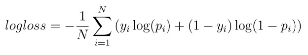
Log loss binary classification: Let’s look at how logloss is calculated. It takes the actual value, 1 or 0, and it takes our prediction, which is a probability between 0 and 1. The greek letter sigma (which looks like an uppercase E below) indicates that we’re taking the sum of the logloss measures for each row of the dataset. We then multiply this sum by -1 over N, the number of rows, to get a single value for loss. We will unpack this math a little more by looking at an example. Consider the case where the true label is 0, but we predict confidently that the label is 1. In this case, because y is 0, the first term becomes 0. This means the logloss is calculated by (1 - y) times log(1 - p). This simplifies to log(1 - 0-point-9) or log(0-point-1), which is 2-point-3. Now, Log loss binary classification: example: consider the case that the correct label is 1, but our model is not sure and our prediction is right in the middle (0-point-5). Our logloss is 0-point-69. Since We are trying to minimize log loss, we can see that it is better to be less confident than it is to be confident and wrong.
- Log loss for binary classi,cation
- Actual value: y = {1=yes, 0=no}
- Prediction (probability that the value is 1): p
- Try label is 0, but we predict confidently that the label is 1
  - logloss = (1 - y) * log(1 - p)
  - logloss = (1 - 0) * log(1 - 0.9)
  - logloss = 2.3
- Try label is 1, but our model is not sure and our prediction is right in the middle (0.5)
  - logloss = -1/N * sum(y * log(p) + (1 - y) * log(1 - p))
  - lobloss = 0.69
  - Better to be less confident than to be confident and wrong
Computing log loss with NumPy: Here is an implementation of logloss. The most important detail is the clip function which sets a maximum and minimum value for the elements in an array. Since log(0) is negative infinity, we want to offset our predictions ever so slightly from being exactly 1 or exactly 0 so that our score remains a real number. In this example we use the eps variable to be 0-point-00 (thirteen zeros) 1, which is close enough to zero to not effect our overall scores. After adjusting the predictions slightly with clip, we calculate logloss using the formula. If we call this function on the examples we looked at earlier, we can see that the confident and wrong item returns the expected value of 2-point-3 and the prediction that is right in the middle returns 0-point-69. We have implemented it here to demonstrate how to take a mathematical equation and turn it into a function to use for evaluation, just like you may need to if you were participating in a machine learning competition.
Let’s practice!: Now let’s develop some intuition for how the logloss metric performs with a few examples.

`def compute_log_loss`

  
def compute_log_loss(predicted: Union[float, List[float]], actual: [int, List[int]], eps: float=1e-14) -> float:
    """
    Computes the logarithmic loss between predicted and 
    actual when these are 1D arrays

    :param predicted: The predicted probabilities as floats between 0-1
    :param actual: The actual binary labels. Either 0 or 1
    :param eps (optional): log(0) is inf, so we need to offset our
                           precidted values slightly by eps from 0 to 1.
    """

    predicted = np.clip(predicted, eps, 1 - eps)
    loss = -1 * np.mean(actual * np.log(predicted)
                        + (1 - actual)
                        * np.log(1 - predicted))
    return loss

  
data = [(0.85, 1), (0.99, 0), (0.51, 0)]

for p, y in data:
    print(compute_log_loss(p, y))

16251892949777494
605170185988091
7133498878774648

Penalizing highly confident wrong answers

As Peter explained in the video, log loss provides a steep penalty for predictions that are both wrong and confident, i.e., a high probability is assigned to the incorrect class.

Suppose you have the following 3 examples:

A: y = 1, p = 0.85
B: y = 0, p = 0.99
C: y = 0, p = 0.51

Select the ordering of the examples which corresponds to the lowest to highest log loss scores. y is an indicator of whether the example was classified correctly. You shouldn’t need to crunch any numbers!

Lowest: A, Middle: C, Highest: B - Of the two incorrect predictions, B will have a higher log loss because it is confident and wrong.

Computing log loss with Numpy

To see how the log loss metric handles the trade-off between accuracy and confidence, we will use some sample data generated with NumPy and compute the log loss using the provided function compute_log_loss(), which Peter showed you in the video.

5 one-dimensional numeric arrays simulating different types of predictions have been pre-loaded: actual_labels, correct_confident, correct_not_confident, wrong_not_confident, and wrong_confident.

Your job is to compute the log loss for each sample set provided using the compute_log_loss(predicted_values, actual_values). It takes the predicted values as the first argument and the actual values as the second argument.

Instructions

Using the compute_log_loss() function, compute the log loss for the following predicted values (in each case, the actual values are contained in actual_labels):
- correct_confident
- correct_not_confident
- wrong_not_confident
- wrong_confident
- actual_labels

  
correct_confident = np.array([0.95, 0.95, 0.95, 0.95, 0.95, 0.05, 0.05, 0.05, 0.05, 0.05])
correct_not_confident = np.array([0.65, 0.65, 0.65, 0.65, 0.65, 0.35, 0.35, 0.35, 0.35, 0.35])
wrong_not_confident = np.array([0.35, 0.35, 0.35, 0.35, 0.35, 0.65, 0.65, 0.65, 0.65, 0.65])
wrong_confident = np.array([0.05, 0.05, 0.05, 0.05, 0.05, 0.95, 0.95, 0.95, 0.95, 0.95])
actual_labels = np.array([1., 1., 1., 1., 1., 0., 0., 0., 0., 0.])

  
# Compute and print log loss for 1st case
correct_confident_loss = compute_log_loss(correct_confident, actual_labels)
print("Log loss, correct and confident: {}".format(correct_confident_loss)) 

# Compute log loss for 2nd case
correct_not_confident_loss = compute_log_loss(correct_not_confident, actual_labels)
print("Log loss, correct and not confident: {}".format(correct_not_confident_loss)) 

# Compute and print log loss for 3rd case
wrong_not_confident_loss = compute_log_loss(wrong_not_confident, actual_labels)
print("Log loss, wrong and not confident: {}".format(wrong_not_confident_loss)) 

# Compute and print log loss for 4th case
wrong_confident_loss = compute_log_loss(wrong_confident, actual_labels)
print("Log loss, wrong and confident: {}".format(wrong_confident_loss)) 

# Compute and print log loss for actual labels
actual_labels_loss = compute_log_loss(actual_labels, actual_labels)
print("Log loss, actual labels: {}".format(actual_labels_loss)) 

Log loss, correct and confident: 0.05129329438755058
Log loss, correct and not confident: 0.4307829160924542
Log loss, wrong and not confident: 1.049822124498678
Log loss, wrong and confident: 2.9957322735539904
Log loss, actual labels: 9.99200722162646e-15

Log loss penalizes highly confident wrong answers much more than any other type. This will be a good metric to use on your models.

Creating a simple first model

In this chapter, you’ll build a first-pass model. You’ll use numeric data only to train the model. Spoiler alert - throwing out all the text data is bad for performance! But you’ll learn how to format your predictions. Then, you’ll be introduced to natural language processing (NLP) in order to start working with the large amounts of text in the data.

It’s time to build a model

It’s time to build a model: When approaching a machine learning problem, and in particular looking at a dataset from a machine learning competition, it’s always a good approach to start with a very simple model. Creating a simple model first helps to give us a sense of how challenging a question actually is. Before we dig deep into complex models where many more things can go wrong, we want to understand how much signal we can pull out using basic methods. We’ll start with a model that just uses the numeric data columns. In building our first model, we want to go from raw data to predictions as quickly as possible. In this case, we’ll use multi-class logistic regression, which treats each label column as independent. The model will train a logistic regression classifier for each of these columns separately and then use those models to predict whether the label appears or not for any given rows. After writing out our predictions to a CSV, we’ll simulate submitting them to the competition and seeing what our score would be.
- Always a good approach to start with a very simple model
- Gives a sense of how challenging the problem is
- Many more things can go wrong in complex models
- How much signal can we pull out using basic methods?
- Train basic model on numeric data only
  - Want to go from raw data to predictions quickly
- Multi-class logistic regression
  - Train classifier of each label separately and use those to predict
- Format predictions and save to CSV
- Compute log loss score of your predictions
Splitting the multi-class dataset: In the supervised learning course, we talked about splitting our data into a training set and a test set. However, because of the nature of our data, the simple approach to a train-test split won’t work. Some labels that only appear in a small fraction of the dataset. If we split our dataset randomly, we may end up with labels in our test set that never appeared in our training set. Our model won’t be able to predict a class that it has never seen before! One approach to this problem is called StratifiedShuffleSplit, which is mentioned in the supervised learning course. However, this scikit-learn function only works if you have a single target variable. In our case, we have many target variables. To work around this issue, we’ve provided a utility function, multilabel_train_test_split, that will ensure that all of the classes are represented in both the test and training sets. We’ll have a link to that code in the exercises if you’re curious.
- Recall: Train-test split
  - Will not work here
  - May end up with labels in test set that never appear in training set
- Solution: StratifiedShuffleSplit
  - Only works with a single target variable
  - We have many target variables
  - multilabel_train_test_split()

Splitting the data: First, we’ll subset our data to just the numeric columns. NUMERIC_COLUMNS is a variable we provide that contains a list of the column names for the columns that are numbers rather than text. Then we’ll do a minimal amount of preprocessing where we fill the NaNs that are in the dataset with -1000. In this case, we choose -1000, because we want our algorithm to respond to NaN’s differently than 0. We’ll create our array of target variables using the get_dummies function in pandas. Again, the get_dummies function takes our categories, and produces a binary indicator for our targets, which is the format that scikit-learn needs to build a model. Finally, we use the multilabel_train_test_split function that is provided to split the dataset in to a training set and a test set.

  
data_to_train = df[NUMERIC_COLUMNS].fillna(-1000)
labels_to_use = pd.get_dummies(df[LABELS])
X_train, X_test, y_train, y_test = multilabel_train_test_split(
 data_to_train,
 labels_to_use,
 size=0.2, seed=123)

Training the model: Now we can import our standard LogisticRegression classifier from sklearn dot linear_model. We’ll also import the OneVsRestClassifier from the sklearn dot multiclass module. OneVsRest let’s us treat each column of y independently. Essentially, it fits a separate classifier for each of the columns. This is just one strategy you can use if you have multiple classes. Take a look at the scikit-learn documentation for other strategies you could consider. Now we can train that classifier by calling fit and passing our features in X_train and the corresponding labels that are in y_train.
1 2 3 4 from sklearn.linear_model import LogisticRegression from sklearn.multiclass import OneVsRestClassifier clf = OneVsRestClassifier(LogisticRegression()) clf.fit(X_train, y_train)
- OneVsRestClassifier:
  - Treats each column of y independently
  - Fits a separate classifier for each of the columns
Let’s practice!: Now it’s your turn to build a model and make some predictions!

Setting up a train-test split in scikit-learn

Alright, you’ve been patient and awesome. It’s finally time to start training models!

The first step is to split the data into a training set and a test set. Some labels don’t occur very often, but we want to make sure that they appear in both the training and the test sets. We provide a function that will make sure at least min_count examples of each label appear in each split: multilabel_train_test_split.

Feel free to check out the full code for multilabel_train_test_split here.

You’ll start with a simple model that uses just the numeric columns of your DataFrame when calling multilabel_train_test_split. The data has been read into a DataFrame df and a list consisting of just the numeric columns is available as NUMERIC_COLUMNS.

  
NUMERIC_COLUMNS_td = df.select_dtypes(include='number').columns.tolist()

# Create the new DataFrame: numeric_data_only
numeric_data_only = df[NUMERIC_COLUMNS_td].fillna(-1000)

# Get labels and convert to dummy variables: label_dummies
label_dummies = pd.get_dummies(df[LABELS_td])

# Create training and test sets
X_train, X_test, y_train, y_test = multilabel_train_test_split(numeric_data_only,
                                                               label_dummies,
                                                               size=0.2, 
                                                               seed=123)

# Print the info
print("X_train info:")
print(X_train.info())
print("\nX_test info:")  
print(X_test.info())
print("\ny_train info:")  
print(y_train.info())
print("\ny_test info:")  
print(y_test.info()) 

X_train info:
<class 'pandas.core.frame.DataFrame'>
Index: 1040 entries, 198 to 101861
Data columns (total 2 columns):
 #   Column  Non-Null Count  Dtype  
---  ------  --------------  -----  
 0   FTE     1040 non-null   float64
 1   Total   1040 non-null   float64
dtypes: float64(2)
memory usage: 24.4 KB
None

X_test info:
<class 'pandas.core.frame.DataFrame'>
Index: 520 entries, 209 to 448628
Data columns (total 2 columns):
 #   Column  Non-Null Count  Dtype  
---  ------  --------------  -----  
 0   FTE     520 non-null    float64
 1   Total   520 non-null    float64
dtypes: float64(2)
memory usage: 12.2 KB
None

y_train info:
<class 'pandas.core.frame.DataFrame'>
Index: 1040 entries, 198 to 101861
Columns: 104 entries, Function_Aides Compensation to Operating_Status_PreK-12 Operating
dtypes: bool(104)
memory usage: 113.8 KB
None

y_test info:
<class 'pandas.core.frame.DataFrame'>
Index: 520 entries, 209 to 448628
Columns: 104 entries, Function_Aides Compensation to Operating_Status_PreK-12 Operating
dtypes: bool(104)
memory usage: 56.9 KB
None


D:\users\trenton\Dropbox\PythonProjects\DataCamp\functions\multilabel.py:31: UserWarning: Size less than number of columns * min_count, returning 520 items instead of 312.0.
  warn(msg.format(y.shape[1] * min_count, size))

Training a model

With split data in hand, you’re only a few lines away from training a model.

In this exercise, you will import the logistic regression and one versus rest classifiers in order to fit a multi-class logistic regression model to the NUMERIC_COLUMNS of your feature data.

Then you’ll test and print the accuracy with the .score() method to see the results of training.

Before you train! Remember, we’re ultimately going to be using logloss to score our model, so don’t worry too much about the accuracy here. Keep in mind that you’re throwing away all of the text data in the dataset - that’s by far most of the data! So don’t get your hopes up for a killer performance just yet. We’re just interested in getting things up and running at the moment.

All data necessary to call multilabel_train_test_split() has been loaded into the workspace.

  
# Instantiate the classifier: clf
clf = OneVsRestClassifier(LogisticRegression())

# Fit the classifier to the training data
clf.fit(X_train, y_train)

# Print the accuracy
print("Accuracy: {}".format(clf.score(X_test, y_test)))

Accuracy: 0.0

The good news is that your workflow didn’t cause any errors. The bad news is that your model scored the lowest possible accuracy: 0.0! But hey, you just threw away ALL of the text data in the budget. Later, you won’t. Before you add the text data, let’s see how the model does when scored by log loss.

Making predictions

Making predictions: Once our classifier is trained, we can use it to make predictions on new data. We could use our test set that we’ve withheld, but we want to simulate actually competing in a data science competition,
Predicting on holdout data: so we will make predictions on the holdout set that the competition provides. As we did with our training data, we load the holdout data using the read_csv function from pandas. We then perform the same simple preprocessing we used earlier. First, we select just the numeric columns. Then we use fillna to replace NaN values with -1000.Finally, we call the predict_proba method on our trained classifier. Remember, we want to predict probabilities for each label, not just whether or not the label appears. If we simply used the predict method instead, we would end up with a 0 or 1 in every case. Because log loss penalizes you for being confident and wrong, the score for this submission would be significantly worse than if we use predict_proba.
1 2 3 houldout = pd.read_csv('HoldoutData.csv', index_col=0) holdout = holdout[NUMERIC_COLUMNS].fillna(-1000) predictions = clf.predict_proba(holdout)

Using .predict()
- would result in an output of 0 or 1
- Log loss penalized being confident and wrong
- Worse performance compared to .predict_proba() 3. Submitting your predictions as a csv: In data science competitions, it’s a standard practice to write your predictions as a CSV and then upload that CSV to the competition platform. From the competition documentation, we can see that the submission format for this competition expects a dataframe that has each of the individual labels as the column headers and probabilities for each of the columns. The to_csv function on a DataFrame, will take our predictions and write them out to a file. One quick note: you’ll notice that our columns have the original column name separated from the value by two underscores. This is because some of the column names already contained single a underscore.

All formatting and submission instructions are provided by the competition

Standard practice to write predictions to a CSV and upload to competition platform
to_csv() method on a DataFrame

Submission format

Each column is an individual label
Each row is a prediction for that label

Write to a file

Format and submit predictions: The predictions that were generated by predict_proba is just an array of values. It doesn’t have column names or an index like our submission format does. We’ll fix this by turning those values into a DataFrame. To get the column names, we use get_dummies on our target variables and then borrow those column names for our new dataframe. Our index will be the same index that we read into pandas with read_csv, and the data is the predictions themselves. As we noted in the previous slide, we want to separate the original column names from the column values with a double underscore when we call get_dummies. To do this, we will use the keyword argument prefix_sep equals double underscore with the get_dummies function. Finally, we can call to_csv and pass the filename of the file we want to write out to disk. We can call the score_submission function that is provided to see how our submission would have scored in the competition!

  
prediction_df = pd.DataFrame(columns=pd.get_dummies(df[LABELS], prefix_sep='__').columns, index=houldout.index, data=predictions)
prediction_df.to_csv('predictions.csv')
score = score_submission(pred_path='predictions.csv')

DrivenData leaderboard: On the DrivenData website, you would submit this CSV file of predictions. We would generate a score for you on the holdout set and then post that score to the leaderboard. Here is an example of the leaderboard from this competition. As the competition proceeds, people make more and more submissions and their place on the leaderboard changes as they build better and better models.

Let’s practice!: Now you’ll get the chance to make some predictions and see what your score is.

Use your model to predict values on holdout data

You’re ready to make some predictions! Remember, the train-test-split you’ve carried out so far is for model development. The original competition provides an additional test set, for which you’ll never actually see the correct labels. This is called the “holdout data.”

The point of the holdout data is to provide a fair test for machine learning competitions. If the labels aren’t known by anyone but DataCamp, DrivenData, or whoever is hosting the competition, you can be sure that no one submits a mere copy of labels to artificially pump up the performance on their model.

Remember that the original goal is to predict the probability of each label. In this exercise you’ll do just that by using the .predict_proba() method on your trained model.

First, however, you’ll need to load the holdout data, which is available in the workspace as the file HoldoutData.csv.

  
# Instantiate the classifier: clf
clf = OneVsRestClassifier(LogisticRegression())

# Fit it to the training data
clf.fit(X_train, y_train)

# Load the holdout data: holdout
holdout = pd.read_csv('data/2024-01-19_school_budgeting_with_machine_learning_in_python/HoldoutData.csv', index_col=0)

# Generate predictions: predictions
NUMERIC_COLUMNS_hd = holdout.select_dtypes(include='number').columns
predictions = clf.predict_proba(holdout[NUMERIC_COLUMNS_hd].fillna(-1000))

Writing out your results to a csv for submission

Writing out your results to a csv for submission At last, you’re ready to submit some predictions for scoring. In this exercise, you’ll write your predictions to a .csv using the .to_csv() method on a pandas DataFrame. Then you’ll evaluate your performance according to the LogLoss metric discussed earlier!

You’ll need to make sure your submission obeys the correct format.

To do this, you’ll use your predictions values to create a new DataFrame, prediction_df.

Interpreting LogLoss & Beating the Benchmark:

When interpreting your log loss score, keep in mind that the score will change based on the number of samples tested. To get a sense of how this very basic model performs, compare your score to the DrivenData benchmark model performance: 2.0455, which merely submitted uniform probabilities for each class.

Remember, the lower the log loss the better. Is your model’s log loss lower than 2.0455?

  
# Format predictions in DataFrame: prediction_df
# pd.get_dummies(df[LABELS], ...) is correctly using df, not holdout
prediction_df = pd.DataFrame(columns=pd.get_dummies(df[LABELS_td], prefix_sep='__').columns,
                             index=holdout.index,
                             data=predictions)

# Save prediction_df to csv
prediction_df.to_csv('data/2024-01-19_school_budgeting_with_machine_learning_in_python/predictions.csv')

  
# requires functions and variables from https://goodboychan.github.io/python/datacamp/machine_learning/2020/06/05/01-School-Budgeting-with-Machine-Learning-in-Python.html
# BOX_PLOTS_COLUMN_INDICES, def _multi_multi_log_loss, and def score_submission

# Submit the predictions for scoring: score
score = score_submission(pred_path='data/2024-01-19_school_budgeting_with_machine_learning_in_python/predictions.csv', holdout_path='data/2024-01-19_school_budgeting_with_machine_learning_in_python/TestSetLabelsSample.csv')

# Print score
print('Your model, trained with numeric data only, yields logloss score: {}'.format(score))

Your model, trained with numeric data only, yields logloss score: 1.9922002736361633

Even though your basic model scored 0.0 accuracy, it nevertheless performs better than the benchmark score of 2.0455. You’ve now got the basics down and have made a first pass at this complicated supervised learning problem. It’s time to step up your game and incorporate the text data.

A very brief introduction to NLP

A very brief introduction to NLP: Some of our data comes in the form or freefrom text. When we have data that is text, we often want to process this text to create features for our algorithms. This is called Natural Language Processing, or NLP. We’ll cover a couple of basic techniques for processing text data. A very brief introduction to NLP: Data for natural language processing can be text, as it is in our case, entire documents (for example, magazine articles or emails), or transcriptions of human speech (like the script I’m reading for this video!). The first step in processing this kind of data is called “tokenization”. Tokenization is the process of splitting a long string into segments. Usually, this means taking a string and splitting it into a list of strings where we have one string for each word. For example, we might split the string “Natural Language Processing” into a list of three separate tokens: “Natural,” “Language,” and “Processing”.
- Data for NLP:
  - Text, documents, speech, …
- Tokenization
  - Splitting a string into segments
  - Store segments as list
- Example: “Natural Language Processing”
  - ['Natural', 'Language', 'Processing']
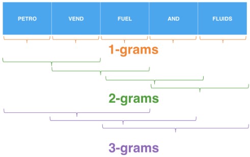
Tokens and token patterns: Let’s take a look at an example of actual data from our school budget dataset. We have the full string “PETRO-VEND FUEL AND FLUIDS.” If we want to tokenize on whitespace, that is split into words every time there is a space, tab, or return in the text, we end up with 4 tokens. The token “PETRO-VEND,” the token “FUEL,” the token “AND,” and the token “FLUIDS.” For some datasets, we may want to split words based on other characters than whitespace. For example, in this dataset we may observe that often we have words that are combined with a hyphen, like “PETRO-VEND.” We can opt in this case to tokenize on whitespace and punctuation. Here we break into tokens every time we see a space or any mark of punctuation. In this case, we end up with 5 tokens: The token “PETRO,” the token “VEND,” the token “FUEL,” the token “AND,” and the token “FLUIDS.” Now that we have our 5 tokens, we want to use them as part of our machine learning algorithm.
- Tokenize on whitespace
  - Petro-vend fuel and fluids
- Petro-vend | fuel | and | fluids - Tokenize on whitespace and punctuation - Petro | vend | fuel | and | fluids
Bag of word presentation: Often, the first way to do this is to simply count the number of times that a particular token appears in a row. This is called a “bag of words” representation, because you can imagine our vocabulary as a bag of all of our words, and we just count the number of times a particular word was pulled out of that bag. If you’re following along closely, you may have noticed that this approach discards information about word order. That is, the phrase “red, not blue” would be treated the same as “blue, not red.” A slightly more sophisticated approach is to create what are called
- Count the number of times a particular token appears
- “Bag of words”
  - Count the number of times a word was pulled out of the bag
- This approach discards information about word order
  - “Red, not blue” is the same as “blue, not red”
1-gram, 2-gram, …, n-gram: “n-grams.” In addition to a column for every token we see, which is called a “1-gram,” we may have a column for every ordered pair of two words. In that case, we’d have a column for “PETRO-VEND,” a column for “VEND FUEL,” a column for “FUEL AND,” and a column for “AND FLUIDS.” These are called 2-grams (or bi-grams). N can be any number, for example, we may also include 3-grams (or tri-grams) in this example. There are three columns for trigrams: one column for “PETRO-VEND FUEL,” one for “VEND FUEL AND,” and one for “FUEL AND FLUIDS.” Now it’s time for a little practice with tokenization and n-grams.
- 1-gram, 2-gram, …, n-gram

Tokenizating text

As we talked about in the video, tokenization is the process of chopping up a character sequence into pieces called tokens.

How do we determine what constitutes a token? Often, tokens are separated by whitespace. But we can specify other delimiters as well. For example, if we decided to tokenize on punctuation, then any punctuation mark would be treated like a whitespace. How we tokenize text in our DataFrame can affect the statistics we use in our model.

A particular cell in our budget DataFrame may have the string content Title I - Disadvantaged Children/Targeted Assistance. The number of n-grams generated by this text data is sensitive to whether or not we tokenize on punctuation, as you’ll show in the following exercise.

How many tokens (1-grams) are in the string

Title I - Disadvantaged Children/Targeted Assistance

if we tokenize on whitespace and punctuation?

Answer

Testing your NLP credentials with n-grams

You’re well on your way to NLP superiority. Let’s test your mastery of n-grams!

In the workspace, we have the loaded a python list, one_grams, which contains all 1-grams of the string petro-vend fuel and fluids, tokenized on punctuation. Specifically,

one_grams = ['petro', 'vend', 'fuel', 'and', 'fluids']

In this exercise, your job is to determine the sum of the sizes of 1-grams, 2-grams and 3-grams generated by the string petro-vend fuel and fluids, tokenized on punctuation.

Recall that the n-gram of a sequence consists of all ordered subsequences of length n.

Answer

12 - The number of 1-grams + 2-grams + 3-grams is 5 + 4 + 3 = 12.

Representing text numerically

Representing text numerically: Let’s talk about how we take the tokenizations we have created and turn them into an array that we can feed into a machine learning algorithm. We mentioned the bag-of-words representation in our last video. This is one of the simplest ways to represent text in a machine learning algorithm. It discards information about grammar and word order, just assuming that the number of times a word occurs is enough information.
- Bag-of-words
  - Simple way to represent text in machine learning
  - Discards information about grammar and word order
  - Computes frequency of occurrence
Scikit-learn tools for bag-of-words: Scikit-learn provides a very useful tool for creating bag-of-words representations. It is called the CountVectorizer. The CountVectorizer works by taking an array of strings and doing three things. First, it tokenizes all of the strings. Then, it makes note of all of the words that appear, which we call the “vocabulary”. Finally, it counts the number of times that each token in the vocabulary appears in every given row.
- CountVectorizer()
  - Tokenizes all the strings
  - Builds a ‘vocabulary’
  - Counts the occurrences of each token in the vocabulary
Using CountVectorizer() on column of main dataset: The CountVectorizer is part of the text submodule in the feature_extraction module in scikit-learn. After importing the CountVectorizer, we will define a regular expression that does a split on whitespace. We won’t go into the details here of how this regular expression works, but there are great resources for learning regular expressions online. We’ll also make sure that our text column does not have any NaN values, simply replacing those with empty strings instead. Finally, we’ll create a CountVectorizer object where we pass in the token_pattern that we have created. This creates an object that we can use to create bag-of-words representations of text. The CountVectorizer object that we’ve created can be used with the fit and transform pattern, just like any other preprocessor in scikit-learn. fit will parse all of the strings for tokens and then create the vocabulary. Here, we use the word vocabulary specifically to mean all of the tokens that appear in this dataset. transform will tokenize the text and then produce the array of counts. As part of the exercises, we’ll look at how changing our token_pattern will change the number of tokens that the CountVectorizer recognizes. ```python from sklearn.feature_extraction.text import CountVecotrizer

TOKENS_BASIC = ‘\\S+(?=\\s+)’ df.Program_Description.fillna(‘’, inplace=True) vec_basic = CountVectorizer(token_pattern=TOKENS_BASIC)

vec_basic.fit(df.Program_Description) msg = ‘There are {} token in Program_Desction if tokean are any non-whitespace’ print(msg.format(len(vec_basic.get_feature_names())))

4. Let's practice!: Now it's time to get some practice using the CountVectorizer from scikit-learn.

### Creating a bag-of-words in scikit-learn

In this exercise, you'll study the effects of tokenizing in different ways by comparing the bag-of-words representations resulting from different token patterns.

You will focus on one feature only, the `Position_Extra` column, which describes any additional information not captured by the `Position_Type` label.

For example, in the Shell you can check out the budget item in row 8960 of the data using `df.loc[8960]`. Looking at the output reveals that this `Object_Description` is overtime pay. For who? The Position Type is merely "other", but the Position Extra elaborates: "BUS DRIVER". Explore the column further to see more instances. It has a lot of NaN values.

Your task is to turn the raw text in this column into a bag-of-words representation by creating tokens that contain only alphanumeric characters.

For comparison purposes, the first 15 tokens of `vec_basic`, which splits `df.Position_Extra` into tokens when it encounters only whitespace characters, have been printed along with the length of the representation.

**Instructions**

- Import `CountVectorizer` from `sklearn.feature_extraction.text`.
- Fill missing values in `df.Position_Extra` using `.fillna('')` to replace NaNs with empty strings. Specify the additional keyword argument `inplace=True` so that you don't have to assign the result back to `df`.
- Instantiate the `CountVectorizer` as `vec_alphanumeric` by specifying the `token_pattern` to be `TOKENS_ALPHANUMERIC`.
- Fit `vec_alphanumeric` to `df.Position_Extra`.
- Hit submit to see the `len` of the fitted representation as well as the first 15 elements, and compare to `vec_basic`.


```python
# Create the token pattern: TOKENS_ALPHANUMERIC
TOKENS_ALPHANUMERIC = '[A-Za-z0-9]+(?=\\s+)'

# Fill missing values in df.Position_Extra
df.fillna({'Position_Extra': ''}, inplace=True)

# Instantiate the CountVectorizer: vec_alphanumeric
vec_alphanumeric = CountVectorizer(token_pattern=TOKENS_ALPHANUMERIC)

# Fit to the data
vec_alphanumeric.fit(df.Position_Extra)

# Print the number of tokens and first 15 tokens
msg = "There are {} tokens in Position_Extra if we split on non-alpha numeric"
print(msg.format(len(vec_alphanumeric.get_feature_names_out())))
print(vec_alphanumeric.get_feature_names_out()[:15])

There are 123 tokens in Position_Extra if we split on non-alpha numeric
['1st' '2nd' '3rd' 'a' 'ab' 'additional' 'adm' 'administrative' 'and'
 'any' 'art' 'assessment' 'assistant' 'asst' 'athletic']

Treating only alpha-numeric characters as tokens gives you a smaller number of more meaningful tokens.

Combining text columns for tokenization

In order to get a bag-of-words representation for all the text data in our DataFrame, you must first convert the text data in each row of the DataFrame into a single string.

In the previous exercise, this wasn’t necessary because you only looked at one column of data, so each row was already just a single string. CountVectorizer expects each row to just be a single string, so in order to use all of the text columns, you’ll need a method to turn a list of strings into a single string.

In this exercise, you’ll complete the function definition combine_text_columns(). When completed, this function will convert all training text data in your DataFrame to a single string per row that can be passed to the vectorizer object and made into a bag-of-words using the .fit_transform() method.

Note that the function uses NUMERIC_COLUMNS and LABELS to determine which columns to drop. These lists have been loaded into the workspace.

Instructions

Use the .drop() method on data_frame with to_drop and axis= as arguments to drop the non-text data. Save the result as text_data.
Fill in missing values (inplace) in text_data with blanks (“”), using the .fillna() method.
Complete the .apply() method by writing a lambda function that uses the .join() method to join all the items in a row with a space in between.

  
# Define combine_text_columns()
def combine_text_columns(data_frame: pd.DataFrame, to_drop: list=NUMERIC_COLUMNS_td + LABELS_td) -> pd.Series:
    """ converts all text in each row of data_frame to single vector """
    
    # Drop non-text columns that are in the df
    to_drop = set(to_drop) & set(data_frame.columns.tolist())
    text_data = data_frame.drop(to_drop, axis=1)
    
    # Replace nans with blanks
    text_data.fillna('', inplace=True)
    
    # Join all text items in a row that have a space in between
    return text_data.apply(lambda x: " ".join(x), axis=1)

What’s in a token?

Now you will use combine_text_columns to convert all training text data in your DataFrame to a single vector that can be passed to the vectorizer object and made into a bag-of-words using the .fit_transform() method.

You’ll compare the effect of tokenizing using any non-whitespace characters as a token and using only alphanumeric characters as a token.

Instructions

Import CountVectorizer from sklearn.feature_extraction.text.
Instantiate vec_basic and vec_alphanumeric using, respectively, the TOKENS_BASIC and TOKENS_ALPHANUMERIC patterns.
Create the text vector by using the combine_text_columns() function on df.
Using the .fit_transform() method with text_vector, fit and transform first vec_basic and then vec_alphanumeric. Print the number of tokens they contain.

  
# Create the basic token pattern
TOKENS_BASIC = '\\S+(?=\\s+)'

# Create the alphanumeric token pattern
TOKENS_ALPHANUMERIC = '[A-Za-z0-9]+(?=\\s+)'

# Instantiate basic CountVectorizer: vec_basic
vec_basic = CountVectorizer(token_pattern=TOKENS_BASIC)

# Instantiate alphanumeric CountVectorizer: vec_alphanumeric
vec_alphanumeric = CountVectorizer(token_pattern=TOKENS_ALPHANUMERIC)

# Create the text vector
text_vector = combine_text_columns(df)

# Fit and transform vec_basic
vec_basic.fit_transform(text_vector)

# Print number of tokens of vec_basic
print("There are {} tokens in the dataset".format(len(vec_basic.get_feature_names_out())))

# Fit and transform vec_alphanumeric
vec_alphanumeric.fit_transform(text_vector)

# Print number of tokens of vec_alphanumeric
print("There are {} alpha-numeric tokens in the dataset".format(len(vec_alphanumeric.get_feature_names_out())))

There are 1406 tokens in the dataset
There are 1118 alpha-numeric tokens in the dataset

Notice that tokenizing on alpha-numeric tokens reduced the number of tokens, just as in the last exercise. We’ll keep this in mind when building a better model with the Pipeline object next.

Improving your model

Here, you’ll improve on your benchmark model using pipelines. Because the budget consists of both text and numeric data, you’ll learn how to build pipelines that process multiple types of data. You’ll also explore how the flexibility of the pipeline workflow makes testing different approaches efficient, even in complicated problems like this one!

Pipelines, feature & text preprocessing

Pipelines, feature & text preprocessing: You’ve submitted your first simple model. Now it’s time to combine what we’ve learned about NLP with our model pipeline and incorporate the text data into our algorithm.
- Repeatable way to go from raw data to trained model
- Pipeline object takes sequential list of steps
  - Output of one step is input to next step
- Each step is a tuple with two elements
  - Name: string
  - Transform: obj implementing .fit() and .transform()
- Flexible: a step can itself be another pipeline!
The pipeline workflow: The supervised learning course introduced pipelines, which are a repeatable way to go from raw data to a trained machine learning model. The scikit-learn Pipeline object takes a sequential list of steps where the output of one step is the input to the next. Each step is represented with a name for the step, that is simply a string, and an object that implements the fit and the transform methods. A good example is the CountVectorizer that we used earlier. As we’ll see Pipelines are a very flexible way to represent your workflow. In fact, you can even have a sub-pipeline as one of the steps! The beauty of the Pipeline is that it encapsulates every transformation from raw data to a trained model.

  
from sklearn.pipeline import Pipeline
from sklearn.linear_model import LogisticRegression
from sklearn.multiclass import OneVsRestClassifier
pl = Pipeline([('clf', OneVsRestClassifier(LogisticRegression()))])

Instantiate simple pipeline with one step: After importing the relevant modules, we’ll start with a one-step pipeline. Although we don’t need a pipeline for a single step, this exercise will get us familiar with the syntax. Remember, we create a Pipeline by passing it a series of named steps. In this case the name is the string ‘clf’, and the step is the one-vs-rest logistic regression classifier we created earlier.
Train and test with sample numeric data: The sample dataset we’ve been working with has numeric data in the numeric columns and the with missing column. We’ll start by building a model to predict the label column with the numeric data.
Train and test with sample numeric data: First, we’ll use the train_test split function from sklearn dot model_selection. Our X will just be the numeric column, and our Y will be the dummy encoding of the label column. We’ll call the fit method on our Pipeline, just like a normal classifier in sklearn. We can see that it returns a Pipeline that has one step to do our logistic regression.

  
from sklearn.model_selection import train_test_split
X_train, X_test, y_train, y_test = train_test_split(sample_df[['numeric']], pd.get_dummies(sample_df['label']), random_state=2)
pl.fit(X_train, y_train)

Train and test with sample numeric data: By using the score function on our pipeline, we can see how our Pipeline performs on the test set. The default scoring method for this classifier is accuracy. That’s good enough for our sample dataset.

  
accuracy = pl.score(X_test, y_test)
print('accuracy on numeric data, no nans: ', accuracy)

Adding more steps to the pipeline: Let’s add the with_missing column to our training set. Oops! Now when we call fit, we see a value error that explains that our input has NaN values.

  
X_train, X_test, y_train, y_test = train_test_split(sample_df[['numeric', 'with_missing']], pd.get_dummies(sample_df['label']), random_state=2)
pl.fit(X_train, y_train)

Preprocessing numeric features with missing data: To address this, we’ll add an Imputer to our pipeline, which will fill in the NaN values. To do so, we add a step to the Pipeline with the name ‘imp’ and an Imputer object. The default imputation in scikit-learn is to fill missing values with the mean of the column in question. You can look at the documentation of the Imputer object to see other possible imputation strategies.

  
from sklearn.preprocessing import Imputer
X_train, X_test, y_train, y_test = train_test_split(sample_df[['numeric', 'with_missing']], pd.get_dummies(sample_df['label']), random_state=2)
pl = Pipeline([('imp', Imputer()), ('clf', OneVsRestClassifier(LogisticRegression()))])

Preprocessing numeric features with missing data: We can call fit and score on the new pipeline, just like we did before. But, in this case our model also includes the column with_missing which had NaN values that were imputed.

  
pipeline.fit(X_train, y_train)
accuracy = pl.score(X_test, y_test)
print('accuracy on all numeric, incl nans: ', accuracy)

Instantiate pipeline

To make your life easier as you start to work with all the data in your original DataFrame, df, it’s time to turn to one of scikit-learn’s most useful objects: the Pipeline.

For the next few exercises, you’ll reacquaint yourself with pipelines and train a classifier on some synthetic (sample) data of multiple datatypes before using the same techniques on the main dataset.

The sample data is stored in the DataFrame, sample_df, which has three kinds of feature data: numeric, text, and numeric with missing values. It also has a label column with two classes, a and b.

In this exercise, your job is to instantiate a pipeline that trains using the numeric column of the sample data.

Instructions

Import Pipeline from sklearn.pipeline.
Create training and test sets using the numeric data only. Do this by specifying sample_df[['numeric']] in train_test_split().
Instantiate a pipeline as pl by adding the classifier step. Use a name of 'clf' and the same classifier from Chapter 2: OneVsRestClassifier(LogisticRegression()).
Fit your pipeline to the training data and compute its accuracy to see it in action! Since this is toy data, you’ll use the default scoring method for now. In the next chapter, you’ll return to log loss scoring.

  
sample_df = pd.read_csv('data/2024-01-19_school_budgeting_with_machine_learning_in_python/sample_df.csv')

sample_df.fillna({'text': ''}, inplace=True)

  
# Split and select numeric data only, no nans 
X_train, X_test, y_train, y_test = train_test_split(sample_df[['numeric']], pd.get_dummies(sample_df['label']),  random_state=22)

# Instantiate Pipeline object: pl
pl = Pipeline([('clf', OneVsRestClassifier(LogisticRegression()))])

# Fit the pipeline to the training data
pl.fit(X_train, y_train)

# Compute and print accuracy
accuracy = pl.score(X_test, y_test)
print("Accuracy on sample data - numeric, no nans: ", accuracy)

Accuracy on sample data - numeric, no nans:  0.62

Now it’s time to incorporate numeric data with missing values by adding a preprocessing step!

Preprocessing numeric features

What would have happened if you had included the with 'with_missing' column in the last exercise? Without imputing missing values, the pipeline would not be happy (try it and see). So, in this exercise you’ll improve your pipeline a bit by using the Imputer() imputation transformer from scikit-learn to fill in missing values in your sample data.

By default, the imputer transformer replaces NaNs with the mean value of the column. That’s a good enough imputation strategy for the sample data, so you won’t need to pass anything extra to the imputer.

After importing the transformer, you will edit the steps list used in the previous exercise by inserting a (name, transform) tuple. Recall that steps are processed sequentially, so make sure the new tuple encoding your preprocessing step is put in the right place.

The sample_df is in the workspace, in case you’d like to take another look. Make sure to select both numeric columns- in the previous exercise we couldn’t use with_missing because we had no preprocessing step!

Instructions

Import Imputer from sklearn.preprocessing.
Create training and test sets by selecting the correct subset of sample_df: numeric and with_missing.
Add the tuple ('imp', Imputer()) to the correct position in the pipeline. Pipeline processes steps sequentially, so the imputation step should come before the classifier step.
Complete the .fit() and .score() methods to fit the pipeline to the data and compute the accuracy.

  
# Create training and test sets using only numeric data
X_train, X_test, y_train, y_test = train_test_split(sample_df[['numeric', 'with_missing']],
                                                    pd.get_dummies(sample_df['label']), 
                                                    random_state=456)

# Insantiate Pipeline object: pl
pl = Pipeline([('imp', SimpleImputer()), ('clf', OneVsRestClassifier(LogisticRegression()))])

# Fit the pipeline to the training data
pl.fit(X_train, y_train)

# Compute and print accuracy
accuracy = pl.score(X_test, y_test)
print("Accuracy on sample data - all numeric, incl nans: ", accuracy)

Accuracy on sample data - all numeric, incl nans:  0.636

Now you know how to use preprocessing in pipelines with numeric data, and it looks like the accuracy has improved because of it! Text data preprocessing is next!

Test features and feature union

Text features and feature unions: In this video, we’ll look at how we process text data in a pipeline and then how we put it all together.
Preprocessing text features: Our sample dataframe contains one column we haven’t used yet, the text column. First, we’ll change our train and test data just to be working with the text data for now. Then, we’ll add a step to our Pipeline with the name vec and the CountVectorizer object from scikit-learn. Now our pipeline will use the CountVectorizer on our dataset, and then it will pass the result into our classifier.

  
from sklearn.feature_extraction.text import CountVectorizer
X_train, X_test, y_train, y_test = train_test_split(sample_df['text'], pd.get_dummies(sample_df['label']), random_state=2)
pl = Pipeline([('vec', CountVectorizer()), ('clf', OneVsRestClassifier(LogisticRegression()))])

Preprocessing text features: Again, we can call the fit and score methods on the Pipeline. The score function now reports our accuracy if we just use the text data.

  
pl.fit(X_train, y_train)

accuracy = pl.score(X_test, y_test)
print('accuracy on sample data: ', accuracy)

Preprocessing multiple dtypes: Let’s say we want to use all of our data in a single pipeline. We can’t just have a Pipeline that has a CountVectorizer step, Imputation step, and then a classifier. The CountVectorizer won’t know what to do with the numeric columns, and we don’t want to perform imputation on the text columns. In order to build our pipeline, we need to separately operate on the text columns and on the numeric columns. There are two tools: FunctionTransformer and FeatureUnion that will help us build a Pipeline to work with both our text and numeric data. The first utility that we cover is the FunctionTransformer.
- Want to use all available features in one pipeline
- Problem
  - Pipeline steps for numeric and text preprocessing can’t follow each other
  - e.g., output of CountVectorizer can’t be input to Imputer
- Solution
  - FunctionTransformer() & FeatureUnion()
FunctionTransformer: FunctionTransformer has a simple job: take a Python function, and turn it into an object that the scikit-learn Pipeline can understand. We’ll write two simple functions: one that takes the whole dataframe, and returns just the numeric columns. The other will take the whole dataframe and return just the text columns. Using these function transformers, we can build a separate Pipeline for our numeric data and for our text data.
- Turns a Python function into an object that a scikit-learn pipeline can understand
- Need to write two functions for pipeline preprocessing
  - Take entire DataFrame, return numeric columns
  - Take entire DataFrame, return text columns
- Can then preprocess numeric and text data in separate pipelines
Putting it all together: First, we’ll do our train_test split on the entire dataset and import the FunctionTransformer and FeatureUnion utilities.

  
X_train, X_test, y_train, y_test = train_test_split(sample_df[['numeric','with_missing', 'text']], pd.get_dummies(sample_df['label']), random_state=2)

from sklearn.preprocessing import FunctionTransformer
from sklearn.pipeline import FeatureUnion

Putting it all together: Next, we’ll create two FunctionTransformer objects. The first takes a dataframe and just returns the column named ‘text’. The second takes a dataframe and returns the columns named ‘numeric’ and ‘with_missing’. These two function transformer objects will let us set up separate Pipelines that operate on the selected columns only. Note that we’ve passed the parameter validate equals False. This simply tells scikit-learn it doesn’t need to check for NaNs or validate the dtypes of the input. We’ll do that work ourselves.

  
get_text_data = FunctionTransformer(lambda x: x['text'], validate=False)
get_numeric_data = FunctionTransformer(lambda x: x[['numeric', 'with_missing']], validate=False)

FeatureUnion Text and Numeric Features: FeatureUnion from the sklearn dot pipeline module is the other utility we need. We know that our text pipeline generates the array on the left, our text features.
FeatureUnion Text and Numeric Features: And our numeric pipeline generates the array on the right, our numeric features.
FeatureUnion Text and Numeric Features: The FeatureUnion object puts these two sets of features together as a single array that will be the input to our classifier.

  
from sklearn.pipeline import FeatureUnion
union = FeatureUnion([('numeric', numeric_pipeline), ('text', text_pipeline)])

Putting it all together: Here’s our entire pipeline, which processes our text and numeric data. First, we create our separate text and numeric pipelines. Remember, get_numeric_data and get_text_data are the FunctionTransformers that we just created. These pipelines output our numeric features and our text features respectively. Then we create our overall pipeline, which has two steps: First, the FeatureUnion takes a list of objects, calls each one, and then concatenates the output into a wide array out of all the results. In this case, it will call our numeric pipeline and then our text pipeline. Once we have this array of all of our features, we can pass it to our classifier. We can call fit and score on this pipeline, just like our simpler ones before it.

  
numeric_pipeline = Pipeline([('selector', get_numeric_data), ('imputer', Imputer())])
text_pipeline = Pipeline([('selector', get_text_data), ('vectorizer', CountVectorizer())])
pl = Pipeline([('union', FeatureUnion([('numeric', numeric_pipeline), ('text', text_pipeline)])),
               ('clf', OneVsRestClassifier(LogisticRegression()))])

Preprocessing text features

Here, you’ll perform a similar preprocessing pipeline step, only this time you’ll use the text column from the sample data.

To preprocess the text, you’ll turn to CountVectorizer() to generate a bag-of-words representation of the data, as in Chapter 2. Using the default arguments, add a (step, transform) tuple to the steps list in your pipeline.

Make sure you select only the text column for splitting your training and test sets.

As usual, your sample_df is ready and waiting in the workspace.

Instructions

Import CountVectorizer from sklearn.feature_extraction.text.
Create training and test sets by selecting the correct subset of sample_df: 'text'.
Add the CountVectorizer step (with the name 'vec') to the correct position in the pipeline.
Fit the pipeline to the training data and compute its accuracy.

  
# Split out only the text data
X_train, X_test, y_train, y_test = train_test_split(sample_df['text'],
                                                    pd.get_dummies(sample_df['label']), 
                                                    random_state=456)

# Instantiate Pipeline object: pl
pl = Pipeline([
        ('vec', CountVectorizer()),
        ('clf', OneVsRestClassifier(LogisticRegression()))
    ])

# Fit to the training data
pl.fit(X_train, y_train)

# Compute and print accuracy
accuracy = pl.score(X_test, y_test)
print("\nAccuracy on sample data - just text data: ", accuracy)

Accuracy on sample data - just text data:  0.808

Multiple types of processing: FunctionTransformer

The next two exercises will introduce new topics you’ll need to make your pipeline truly excel.

Any step in the pipeline must be an object that implements the fit and transform methods. The FunctionTransformer creates an object with these methods out of any Python function that you pass to it. We’ll use it to help select subsets of data in a way that plays nicely with pipelines.

You are working with numeric data that needs imputation, and text data that needs to be converted into a bag-of-words. You’ll create functions that separate the text from the numeric variables and see how the .fit() and .transform() methods work.

Instructions

Compute the selector get_text_data by using a lambda function and FunctionTransformer() to obtain all 'text' columns.
Compute the selector get_numeric_data by using a lambda function and FunctionTransformer() to obtain all the numeric columns (including missing data). These are 'numeric' and 'with_missing'.
Fit and transform get_text_data using the .fit_transform() method with sample_df as the argument.
Fit and transform get_numeric_data using the same approach as above.

  
# Obtain the text data: get_text_data
get_text_data = FunctionTransformer(lambda x: x['text'], validate=False)

# Obtain the numeric data: get_numeric_data
get_numeric_data = FunctionTransformer(lambda x: x[['numeric', 'with_missing']], validate=False)

# Fit and transform the text data: just_text_data
just_text_data = get_text_data.fit_transform(sample_df)

# Fit and transform the numeric data: just_numeric_data
just_numeric_data = get_numeric_data.fit_transform(sample_df)

# Print head to check results
print('Text Data')
display(just_text_data.head())
print('\nNumeric Data')
display(just_numeric_data.head())

Text Data

0           
1        foo
2    foo bar
3           
4    foo bar
Name: text, dtype: object

Numeric Data

	numeric	with_missing
0	-10.856306	4.433240
1	9.973454	4.310229
2	2.829785	2.469828
3	-15.062947	2.852981
4	-5.786003	1.826475

Multiple types of processing: FeatureUnion

Now that you can separate text and numeric data in your pipeline, you’re ready to perform separate steps on each by nesting pipelines and using FeatureUnion().

These tools will allow you to streamline all preprocessing steps for your model, even when multiple datatypes are involved. Here, for example, you don’t want to impute our text data, and you don’t want to create a bag-of-words with our numeric data. Instead, you want to deal with these separately and then join the results together using FeatureUnion().

In the end, you’ll still have only two high-level steps in your pipeline: preprocessing and model instantiation. The difference is that the first preprocessing step actually consists of a pipeline for numeric data and a pipeline for text data. The results of those pipelines are joined using FeatureUnion().

Instructions

In the process_and_join_features:
- Add the steps ('selector', get_numeric_data) and ('imputer', Imputer()) to the 'numeric_features' preprocessing step.
- Add the equivalent steps for the text_features preprocessing step. That is, use get_text_data and a CountVectorizer step with the name 'vectorizer'.
Add the transform step process_and_join_features to 'union' in the main pipeline, pl.
Hit submit to see the pipeline in action!

  
# Split using ALL data in sample_df
X_train, X_test, y_train, y_test = train_test_split(sample_df[['numeric', 'with_missing', 'text']],
                                                    pd.get_dummies(sample_df['label']), 
                                                    random_state=22)

# Create a FeatureUnion with nested pipeline: process_and_join_features
process_and_join_features = FeatureUnion(
            transformer_list = [
                ('numeric_features', Pipeline([
                    ('selector', get_numeric_data),
                    ('imputer', SimpleImputer())
                ])),
                ('text_features', Pipeline([
                    ('selector', get_text_data),
                    ('vectorizer', CountVectorizer())
                ]))
             ]
        )

# Instantiate nested pipeline: pl
pl = Pipeline([
        ('union', process_and_join_features),
        ('clf', OneVsRestClassifier(LogisticRegression()))
    ])


# Fit pl to the training data
pl.fit(X_train, y_train)

# Compute and print accuracy
accuracy = pl.score(X_test, y_test)
print("\nAccuracy on sample data - all data: ", accuracy)

Accuracy on sample data - all data:  0.928

Choosing a classification model

Choosing a classification model: Now that we understand how to pull together text and numeric data into a single machine learning pipeline, we’ll return to talking about our school budget dataset. In the sample dataset, there was only one text column. This is the format that CountVectorizer expects.
Main dataset: lots of text: However, our main dataset has 14 text columns. In an interactive exercise during our NLP chapter we wrote a function combine_text_columns that put together all the text columns into a single column. We’ll re-use this function as part of our Pipeline to process the text in the budget dataset.

  
LABELS = ['Function', 'Use', 'Sharing', 'Reporting', 'Student_Type', 'Position_Type', 'Object_Type', 'Pre_K', 'Operating_Status']
NON_LABELS = [c for c in df.columns if c not in LABELS]
len(NON_LABELS) - len(NUMERIC_COLUMNS)

Using pipeline with the main dataset: Again, as we did in the last chapter, we’ll use the get_dummies function from pandas to create our label array, and we’ll also create our train-test split using the multilabel_train_test_split function. Hopefully, this is starting to feel familiar.
Using pipeline with the main dataset: Now we’ll create a pipeline for working with our main dataset. The beauty of this code, is that it has one change from the code we used for the sample dataset: we create a FunctionTransformer object using our combine_text_columns function instead of the simple selection function we used in the sample dataset. Other than this one change, the pipeline that processes the text, imputes the numeric columns, joins those results together and then fits a multilabel logistic regression remains the same.

  
import numpy as np
import pandas as pd

df = pd.read_csv('TrainingSetSample.csv', index_col=0)
dummy_labels = pd.get_dummies(df[LABELS])
X_train, X_test, y_train, y_test = multilabel_train_test_split(
    df[NON_LABELS], dummy_labels,
    0.2)

get_text_data = FunctionTransformer(combine_text_columns, validate=False)
get_numeric_data = FunctionTransformer(lambda x: x[NUMERIC_COLUMNS], validate=False)
pl = Pipeline([
    ('union', FeatureUnion([
        ('numeric_features', Pipeline([
            ('selector', get_numeric_data),
            ('imputer', Imputer())
        ])),
        ('text_features', Pipeline([
            ('selector', get_text_data),
            ('vectorizer', CountVectorizer())
        ]))
    ])
     ),
    ('clf', OneVsRestClassifier(LogisticRegression()))
])

Performance using main dataset: We can now fit this Pipeline on the school budget dataset. As part of our exercises, we’ll look at the results of this pipeline. Now we have infrastructure for processing our features and fitting a model. This infrastructure allows us to easily experiment with adapting different parts of the pipeline. Part of your challenge in the exercises will be to improve the performance of the pipeline.

  
pl.fit(X_train, y_train)

Flexibility of model step: For example, we can easily experiment with different classes of models. All of our Pipeline code can stay the same, but we can update the last step to be a different class of model instead of LogisticRegression. For example, we could try a RandomForestClassifier, NaiveBayesClassifier, or a KNeighborsClassifier instead. In fact, you can look at the scikit-learn documentation and choose any model class you want!
- Is current model the best?
- Can quickly try different models with pipelines
  - Pipeline preprocessing steps unchanged
  - Edit the model step in your pipeline
  - Random Forest, Naive Bayes, k-NN
Easily try new models using pipeline: Here’s an example of how simple it is to change the classification method in our scikit-learn Pipeline. We simply import a different class of model–in this case, we’ll use a RandomForestClassifier. Then, the only other line that needs to change is the one that defines the classifier inside the Pipeline. This makes it very simple for us to try a large number of different model classes and determine which one is the best for the problem that we’re working on.

  
from sklearn.ensemble import RandomForestClassifier

pl = Pipeline([
    ('union', FeatureUnion(
        transformer_list=[
            ('numeric_features', Pipeline([
                ('selector', get_numeric_data),
                ('imputer', Imputer())
            ])),
            ('text_features', Pipeline([
                ('selector', get_text_data),
                ('vectorizer', CountVectorizer())
            ]))
        ]
    )),
    ('clf', OneVsRest(RandomForestClassifier()))
])

Let’s practice: Now your task is to implement the classification pipeline on the school budget dataset. You will also get the chance to experiment with the Pipeline steps and model class. See how much you can improve the performance of the model!

Using FunctionTransformer on the main dataset

In this exercise you’re going to use FunctionTransformer on the primary budget data, before instantiating a multiple-datatype pipeline in the next exercise.

Recall from Chapter 2 that you used a custom function combine_text_columns to select and properly format text data for tokenization; it is loaded into the workspace and ready to be put to work in a function transformer!

Concerning the numeric data, you can use NUMERIC_COLUMNS, preloaded as usual, to help design a subset-selecting lambda function.

You’re all finished with sample data. The original df is back in the workspace, ready to use.

Instructions

Complete the call to multilabel_train_test_split() by selecting df[NON_LABELS].
Compute get_text_data by using FunctionTransformer() and passing in combine_text_columns. Be sure to also specify validate=False.
Use FunctionTransformer() to compute get_numeric_data. In the lambda function, select out the NUMERIC_COLUMNS of x. Like you did when computing get_text_data, also specify validate=False.

  
df = pd.read_csv('data/2024-01-19_school_budgeting_with_machine_learning_in_python/TrainingData.csv', index_col=0)
LABELS_td = ['Function', 'Use', 'Sharing', 'Reporting', 'Student_Type', 'Position_Type', 'Object_Type', 'Pre_K', 'Operating_Status']
categorize_label = lambda x: x.astype('category')
df[LABELS_td] = df[LABELS_td].apply(categorize_label)
NUMERIC_COLUMNS_td = df.select_dtypes(include='number').columns.tolist()

  
# Get the dummy encoding of the labels
dummy_labels = pd.get_dummies(df[LABELS_td])

# Get the columns that are features in the original df
NON_LABELS = [c for c in df.columns if c not in LABELS_td]

# Split into training and test sets
X_train, X_test, y_train, y_test = multilabel_train_test_split(df[NON_LABELS],
                                                               dummy_labels,
                                                               0.2, 
                                                               seed=123)

# Preprocess the text data: get_text_data
get_text_data = FunctionTransformer(combine_text_columns, validate=False)

# Preprocess the numeric data: get_numeric_data
get_numeric_data = FunctionTransformer(lambda x: x[NUMERIC_COLUMNS_td], validate=False)

D:\users\trenton\Dropbox\PythonProjects\DataCamp\functions\multilabel.py:31: UserWarning: Size less than number of columns * min_count, returning 520 items instead of 312.0.
  warn(msg.format(y.shape[1] * min_count, size))

Add a model to the pipeline

You’re about to take everything you’ve learned so far and implement it in a Pipeline that works with the real, DrivenData budget line item data you’ve been exploring.

Surprise! The structure of the pipeline is exactly the same as earlier in this chapter:

the preprocessing step uses FeatureUnion to join the results of nested pipelines that each rely on FunctionTransformer to select multiple datatypes
the model step stores the model object
You can then call familiar methods like .fit() and .score() on the Pipeline object pl.

Instructions

Complete the 'numeric_features' transform with the following steps:
- get_numeric_data, with the name 'selector'.
- Imputer(), with the name 'imputer'.
Complete the 'text_features' transform with the following steps:
- get_text_data, with the name 'selector'.
- CountVectorizer(), with the name 'vectorizer'.
Fit the pipeline to the training data.
Hit submit to compute the accuracy!

  
# Complete the pipeline: pl
pl = Pipeline([
        ('union', FeatureUnion(
            transformer_list = [
                ('numeric_features', Pipeline([
                    ('selector', get_numeric_data),
                    ('imputer', SimpleImputer())
                ])),
                ('text_features', Pipeline([
                    ('selector', get_text_data),
                    ('vectorizer', CountVectorizer())
                ]))
             ]
        )),
        ('clf', OneVsRestClassifier(LogisticRegression(max_iter=1000)))
    ])

# Fit to the training data
pl.fit(X_train, y_train)

# Compute and print accuracy
accuracy = pl.score(X_test, y_test)
print("\nAccuracy on budget dataset: ", accuracy)

Accuracy on budget dataset:  0.0

Now that you’ve built the entire pipeline, you can easily start trying out different models by just modifying the 'clf' step.

Try a different class of model

Now you’re cruising. One of the great strengths of pipelines is how easy they make the process of testing different models.

Until now, you’ve been using the model step ('clf', OneVsRestClassifier(LogisticRegression())) in your pipeline.

But what if you want to try a different model? Do you need to build an entirely new pipeline? New nests? New FeatureUnions? Nope! You just have a simple one-line change, as you’ll see in this exercise.

In particular, you’ll swap out the logistic-regression model and replace it with a random forest classifier, which uses the statistics of an ensemble of decision trees to generate predictions.

Instructions

Import the RandomForestClassifier from sklearn.ensemble.
Add a RandomForestClassifier() step named 'clf' to the pipeline.
Hit submit to fit the pipeline to the training data and compute its accuracy.

  
# Edit model step in pipeline
pl = Pipeline([
        ('union', FeatureUnion(
            transformer_list = [
                ('numeric_features', Pipeline([
                    ('selector', get_numeric_data),
                    ('imputer', SimpleImputer())
                ])),
                ('text_features', Pipeline([
                    ('selector', get_text_data),
                    ('vectorizer', CountVectorizer())
                ]))
             ]
        )),
        ('clf', RandomForestClassifier(n_jobs=-1))
    ])

# Fit to the training data
pl.fit(X_train, y_train)

# Compute and print accuracy
accuracy = pl.score(X_test, y_test)
print("\nAccuracy on budget dataset: ", accuracy)

Accuracy on budget dataset:  0.325

An accuracy improvement- amazing! All your work building the pipeline is paying off. It’s now very simple to test different models!

Can you adjust the model or parameters to improve accuracy?

You just saw a substantial improvement in accuracy by swapping out the model. Pipelines are amazing!

Can you make it better? Try changing the parameter n_estimators of RandomForestClassifier(), whose default value is 10, to 15.

  
# Edit model step in pipeline
pl = Pipeline([
        ('union', FeatureUnion(
            transformer_list = [
                ('numeric_features', Pipeline([
                    ('selector', get_numeric_data),
                    ('imputer', SimpleImputer())
                ])),
                ('text_features', Pipeline([
                    ('selector', get_text_data),
                    ('vectorizer', CountVectorizer())
                ]))
             ]
        )),
        ('clf', RandomForestClassifier(n_estimators=15, n_jobs=-1))
    ])

# Fit to the training data
pl.fit(X_train, y_train)

# Compute and print accuracy
accuracy = pl.score(X_test, y_test)
print("\nAccuracy on budget dataset: ", accuracy)

Accuracy on budget dataset:  0.3076923076923077

It’s time to get serious and work with the log loss metric. You’ll learn expert techniques in the next chapter to take the model to the next level.

Learning from the experts

In this chapter, you will learn the tricks used by the competition winner, and implement them yourself using scikit-learn.

Learning from the expert: processing

Learning from the expert: processing: In this chapter, we’re going to see the tips and tricks that got the winning competitor to the top of the leaderboard.
Learning from the expert: Some tricks are about text processing, some are about statistical methods, and some are about computational efficiency. While some of this may be new, some of it may be familiar from this course or other work you’ve done on DataCamp. By knowing which tools to combine, we can build extremely effective models.
- Text processing
- Statistical methods
- Computational efficiency
Learning from the expert: text preprocessing: In our introduction to natural language processing, we introduced the same tools that the winner used. These are common tools for manipulating text, and are often effective for improving models based on text data. The first trick the winner used was to tokenize on punctuation. By noticing that there are lots of characters like hyphens, periods, and underscores in the text we are working with, the winner picked out a better way of separating words than just spaces. The other trick was to use a range of n-grams in the model. By including unigrams and bigrams, the winner was more likely to capture important information that appears as multiple tokens in the text–for example, “middle school.”
- NLP tricks for text data
  - Tokenize on punctuation to avoid hyphens, underscores, etc.
  - Include unigrams and bi-grams in the model to capture important information involving multiple tokens (e.g., “middle school”)
N-grams and tokenization: One of the massive benefits of building our models on top of scikit-learn is that many of these common tools are implemented for us and are well-tested by a large community. To change our tokenization and add bi-grams, we can change our call to CountVectorizer. We’ll pass the regular expression to only accept alphanumeric characters in our tokens. We defined this expression back in chapter 2. We’ll also add the parameter ngram_range equals (1, 2). This tells the CountVectorizer to include 1-grams and 2-grams in the vectorization. These changes to the call to CountVectorizer are the only changes we need to make to add these preprocessing steps. We can easily update our pipeline to include this change, which will be part of the exercises.
1 vec = CountVectorizer(token_pattern=TOKENS_ALPHANUMERIC, ngram_range=(1, 2))
- Simple changes to CountVectorizer can improve your model
  - token_pattern parameter to avoid breaking on hyphens
  - ngram_range parameter to include unigrams and bigrams
- ngram_range=(min_n, max_n) - alphanumeric tokenization
- token_pattern=TOKENS_ALPHANUMERIC
Range of n-grams in scikit-learn: Then we fit our updated pipeline in the same way that we’ve been doing throughout the course: call the fit method on our Pipeline object. Getting predictions from our model is also the same as it has been throughout.
Range of n-grams in scikit-learn: We use the predict_proba function to get our class probabilities. Because we have built our preprocessing into our Pipeline, we don’t need to do any additional processing on our holdout data when we load it. The pipeline represents the entire prediction process from raw data to class probabilities. ```python pl.fit(X_train, y_train)

holdout = pd.read_csv(‘HoldoutData.csv’, index_col=0) predictions = pl.predict_proba(holdout) prediction_df = pd.DataFrame(columns=pd.get_dummies( df[LABELS]).columns, index=holdout.index, data=predictions) prediction_df.to_csv(‘predictions.csv’) score = score_submission(pred_path=’predictions.csv’)

7. Let's practice!: Now it's your turn to implement these text processing tricks and see how they improve your score.


```python
df = pd.read_csv('data/2024-01-19_school_budgeting_with_machine_learning_in_python/TrainingData.csv', index_col=0)
LABELS_td = ['Function', 'Use', 'Sharing', 'Reporting', 'Student_Type', 'Position_Type', 'Object_Type', 'Pre_K', 'Operating_Status']
categorize_label = lambda x: x.astype('category')
df[LABELS_td] = df[LABELS_td].apply(categorize_label)
NUMERIC_COLUMNS_td = df.select_dtypes(include='number').columns.tolist()

How many tokens?

Recall from previous chapters that how you tokenize text affects the n-gram statistics used in your model.

Going forward, you’ll use alphanumeric sequences, and only alphanumeric sequences, as tokens. Alphanumeric tokens contain only letters a-z and numbers 0-9 (no other characters). In other words, you’ll tokenize on punctuation to generate n-gram statistics.

In this exercise, you’ll make sure you remember how to tokenize on punctuation.

Assuming we tokenize on punctuation, accepting only alphanumeric sequences as tokens, how many tokens are in the following string from the main dataset?

'PLANNING,RES,DEV,& EVAL ' If you want, we’ve loaded this string into the workspace as SAMPLE_STRING, but you may not need it to answer the question.

Instructions

~~4, because RES and DEV are not tokens~~
4, because , and & are not tokens - Commas, “&”, and whitespace are not alphanumeric tokens.
~~7, because there are 4 different words, some commas, an & symbol, and whitespace~~
~~7, because there are 7 whitespaces~~

Deciding what’s a word

Before you build up to the winning pipeline, it will be useful to look a little deeper into how the text features will be processed.

In this exercise, you will use CountVectorizer on the training data X_train (preloaded into the workspace) to see the effect of tokenization on punctuation.

Remember, since CountVectorizer expects a vector, you’ll need to use the preloaded function, combine_text_columns before fitting to the training data.

Instructions

Create text_vector by preprocessing X_train using combine_text_columns. This is important, or else you won’t get any tokens!
Instantiate CountVectorizer as text_features. Specify the keyword argument token_pattern=TOKENS_ALPHANUMERIC.
Fit text_features to the text_vector.
Hit submit to print the first 10 tokens.

  
# Create the text vector
text_vector = combine_text_columns(X_train)

# Create the token pattern: TOKENS_ALPHANUMERIC
TOKENS_ALPHANUMERIC = '[A-Za-z0-9]+(?=\\s+)'

# Instantiate the CountVectorizer: text_features
text_features = CountVectorizer(token_pattern=TOKENS_ALPHANUMERIC)

# Fit text_features to the text vector
text_features.fit(text_vector)

# Print the first 10 tokens
print(text_features.get_feature_names_out()[:10])

['00a' '12' '1st' '2nd' '4th' '5th' '70h' '8' 'a' 'aaps']

N-gram range in scikit-learn

In this exercise, you’ll insert a CountVectorizer instance into your pipeline for the main dataset, and compute multiple n-gram features to be used in the model.

To look for ngram relationships at multiple scales, you will use the ngram_range parameter as Peter discussed in the video.

Special functions: You’ll notice a couple of new steps provided in the pipeline in this and many of the remaining exercises. Specifically, the dim_red step following the vectorizer step, and the scale step preceding the clf (classification) step.

These have been added to account for the fact that you’re using a reduced-size sample of the full dataset in this course. To make sure the models perform as the expert competition winner intended, we have to apply a dimensionality reduction technique, which is what the dim_red step does. We have to scale the features to lie between -1 and 1, which is what the scale step does.

The dim_red step uses a scikit-learn function called SelectKBest(), applying something called the chi-squared test to select the K “best” features. The scale step uses a scikit-learn function called MaxAbsScaler() to squash the relevant features into the interval -1 to 1.

You won’t need to do anything extra with these functions here, complete the vectorizing pipeline steps below. However, notice how easy it was to add more processing steps to our pipeline!

Instructions

Import CountVectorizer from sklearn.feature_extraction.text.
Add a CountVectorizer step to the pipeline with the name 'vectorizer'.
Set the token pattern to be TOKENS_ALPHANUMERIC.
Set the ngram_range to be (1, 2).

  
# Select 300 best features
chi_k = 300

# Perform preprocessing
get_text_data = FunctionTransformer(combine_text_columns, validate=False)
get_numeric_data = FunctionTransformer(lambda x: x[NUMERIC_COLUMNS_td], validate=False)

# Create the token pattern: TOKENS_ALPHANUMERIC
TOKENS_ALPHANUMERIC = '[A-Za-z0-9]+(?=\\s+)'

# Instantiate pipeline: pl
pl = Pipeline([
        ('union', FeatureUnion(
            transformer_list = [
                ('numeric_features', Pipeline([
                    ('selector', get_numeric_data),
                    ('imputer', SimpleImputer())
                ])),
                ('text_features', Pipeline([
                    ('selector', get_text_data),
                    ('vectorizer', CountVectorizer(token_pattern=TOKENS_ALPHANUMERIC, ngram_range=(1, 2))),
                    ('dim_red', SelectKBest(chi2, k=chi_k))
                ]))
             ]
        )),
        ('scale', MaxAbsScaler()),
        ('clf', OneVsRestClassifier(LogisticRegression()))
    ])

# fit the pipeline to our training data
pl.fit(X_train, y_train.values)

# print the score of our trained pipeline on our test set
log_loss_scorer = make_scorer(_multi_multi_log_loss)
print("Logloss score of trained pipeline: ", log_loss_scorer(pl, X_test, y_test.values))

Logloss score of trained pipeline:  3.1193204946981092

Learning from the expert: a stats trick

Learning from the expert: a stats trick: Now that you have experience with the text processing tricks that won the competition, we’ll introduce some additional tools that the winner used.
Learning from the expert: interaction terms: The statistical tool that the winner used is called interaction terms. We use bigrams to account for when words appear in a certain order. However, what if terms are not next to each other? For example, consider “English Teacher for 2nd Grade” and “2nd Grade - budget for English Teacher”. If I want to identify this line item as a staff position for an elementary school, it helps to know that both “2nd grade” and “English teacher” appear. Interaction terms let us mathematically describe when tokens appear together.
- Statistical tool that the winner used: interaction terms
- Example
  - English teacher for 2nd grade
  - 2nd grade - budget for English teacher
- Interaction terms mathematically describe when tokens appear together
Interaction terms: the math: We’re going to walk through a brief bit of math here to help explain interaction terms. If we look at a simple linear model, we have
Interaction terms: the math: Beta-one times X1, beta 2 times X2.
Interaction terms: the math: Here, X1 and X2 represent whether a particular token appears in the row. The betas are the coefficients, which represent how important that particular token is. To add an interaction term,
Interaction terms: the math: we add another column to our array, X3 that equals X1 times X2. Because X1 and X2 are either 0 or 1, when we multiply them, we only get a 1 if both occur. This new column, X3, has its own coefficient, Beta 3, which can separately measure how important it is that X1 and X2 appear together. Again,
Adding interaction features with scikit-learn: scikit-learn provides us with a straightforward way of adding interaction terms. In scikit-learn this functionality is called PolynomialFeatures, and we import it from the sklearn dot preprocessing module. As an example, we’ll show the same x matrix as the last slide. When we create a PolynomialFeatures we tell it the degree of features to include. In our example, we looked at multiplying 2 columns together to see if they co-occurred, so degree equals 2, however, you could 3, 4, or more. While this can sometimes improve the model results, adding larger degrees very quickly scales the number of features outside what is computationally feasible. The interaction_only equals True parameter tells PolynomialFeatures that we don’t need to multiply a column by itself, and we’ll talk about include_bias on the next slide. When we fit and transform our array, x, we can see that we get the expected output from the last slide with the new column added. We opted not to include a bias term in our model, but you could have if you wanted to. A bias term is an offset for a model.

  
from sklearn.preprocessing import PolynomialFeatures

x = pd.DataFrame({'x1': [0, 1], 'x2': [1, 1]})

interaction = PolynomialFeatures(degree=2,
                                 interaction_only=True,
                                 include_bias=False)
interaction.fit_transform(x)

[out]:
array([[0., 1., 0.],
       [1., 1., 1.]])

A note about bias terms: For example, if we plot age on the x-axis, and weights on the y-axis, we’d have a line that had a value 7-point-5 lbs when the baby is born, because a baby has a weight even when it is 0 years old! A bias term allows your model to account for situations where an x value of 0 should have a y value that is not 0, like in this example.
- Bias term allows your model to have non-zero y value when x is 0
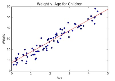
Sparse interaction features: As we mentioned, adding interaction terms makes your X array grow exponentially. Because of computational concerns, our CountVectorizer returns an object called a sparse matrix. We won’t dig into the details here, but the standard PolynomialFeatures object is not compatible with a sparse matrix. We provide you with a replacement, SparseInteractions which works with a sparse matrix. You only need to pass it the degree parameter for it to work in the same way.
- SparseInteractions(degree=2).fit_transform(x).toarray()
- The number of interaction terms grows exponentially
- Our vectorizer saves memory by using a sparse matrix
- PolynomialFeatures does not support sparse matrices
- We have provided SparseInteractions to work for this problem
Let’s practice!: Now it’s your turn to practice adding interaction terms with SparseInteractions to your code, and you can see what effect they have on your score!

Which models of the data include interaction terms?

Recall from the video that interaction terms involve products of features.

Suppose we have two features x and y, and we use models that process the features as follows:

βx + βy + ββ
βxy + βx + βy
βx + βy + βx^2 + βy^2

where β is a coefficient in your model (not a feature).

Which expression(s) include interaction terms?

Answer the question

~~The first expression.~~
The second expression. - The second expression includes the interaction term βxy, where the xy term is present, which represents interactions between features
~~The third expression.~~
~~The first and third expressions.~~

Implement interaction modeling in scikit-learn

It’s time to add interaction features to your model. The PolynomialFeatures object in scikit-learn does just that, but here you’re going to use a custom interaction object, SparseInteractions. Interaction terms are a statistical tool that lets your model express what happens if two features appear together in the same row.

SparseInteractions does the same thing as PolynomialFeatures, but it uses sparse matrices to do so. You can get the code for SparseInteractions at this GitHub Gist.

PolynomialFeatures and SparseInteractions both take the argument degree, which tells them what polynomial degree of interactions to compute.

You’re going to consider interaction terms of degree=2 in your pipeline. You will insert these steps after the preprocessing steps you’ve built out so far, but before the classifier steps.

Pipelines with interaction terms take a while to train (since you’re making n features into n-squared features!), so as long as you set it up right, we’ll do the heavy lifting and tell you what your score is!

Instructions

Add the interaction terms step using SparseInteractions() with degree=2. Give it a name of 'int', and make sure it is after the preprocessing step but before scaling.

  
# Instantiate pipeline: pl
pl = Pipeline([
    ('union', FeatureUnion(
        transformer_list=[
            ('numeric_features', Pipeline([
                ('selector', get_numeric_data),
                ('imputer', SimpleImputer())
            ])),
            ('text_features', Pipeline([
                ('selector', get_text_data),
                ('vectorizer', CountVectorizer(token_pattern=TOKENS_ALPHANUMERIC,
                                               ngram_range=(1, 2))),
                ('dim_red', SelectKBest(chi2, k=chi_k))
            ]))
        ]
    )),
    ('int', SparseInteractions(degree=2)),
    ('scale', MaxAbsScaler()),
    ('clf', OneVsRestClassifier(LogisticRegression()))
])

# fit the pipeline to our training data
pl.fit(X_train, y_train.values)

# print the score of our trained pipeline on our test set
log_loss_scorer = make_scorer(_multi_multi_log_loss)
print("Logloss score of trained pipeline: ", log_loss_scorer(pl, X_test, y_test.values))

Logloss score of trained pipeline:  3.640359198540859

Learning from the expert: the winning model

Learning from the expert: the winning model: Congratulations! You’ve implemented nearly all of the winning pipeline. Just a couple more tweaks.
Learning from the expert: hashing trick: We’ve mentioned that we need to balance adding new features with the computational cost of additional columns. For example, adding 3-grams or 4-grams is going to have an enormous increase in the size of the array. As the array grows in size, we need more computational power to fit our model. The “hashing trick” is a way of limiting the size of the matrix that we create without sacrificing too much model accuracy. A hash function takes an input, in this case a token, and outputs a hash value. For example, the hash value may be an integer like in this example below. We explicitly state how many possible outputs the hashing function may have. For example, we may say that we will only have 250 outputs of the hash function. The HashingVectorizer then maps every token to one of those 250 columns. Some columns will have multiple tokens that map to them. Interestingly, the original paper about the hashing function demonstrates that even if two tokens hash to the same value, there is very little effect on model accuracy in real world problems.
- Adding new features may cause enormous increase in array size
- Hashing is a way of increasing memory efficiency
- Hash function limits possible outputs, fixing array size
When to use the hashing trick: We’ve been working with a small subset of the data for this course, however, the size of the full dataset is part of the challenge. In this situation, we want to do whatever we can to make our array of features smaller. Doing so is called “dimensionality reduction”. The hashing trick is particularly useful in cases like this where we have a very large amount of text data.
- Want to make array of features as small as possible
  - Dimensionality reduction
  - Particularly useful on large datasets
  - e.g., lots of text data!
Implementing the hashing trick in scikit-learn: Implementing the hashing trick is very simple in scikit-learn. Instead of using the CountVectorizer, which creates the bag of words representation, we change to the HashingVectorizer. We can pass this the same token_pattern and ngram_range as before. The parameters norm equals None and non_negative equals True let you drop in the HashingVectorizer as a replacement for the CountVectorizer. For more details on those two parameters, you can see the scikit-learn documentation. We can now use the HashingVectorizer in a Pipeline instead of the CountVectorizer.
1 2 from sklearn.feature_extraction.text import HashingVectorizer vec = HashingVectorizer(norm=None, non_negative=True, token_pattern=TOKENS_ALPHANUMERIC, ngram_range=(1, 2))
The model that won it all: We’ve worked through the three categories of tools that the winner put together to win the competition. The NLP trick was to use bigrams and tokenize on punctuation. The statistical trick was to add interaction terms to the model. The computational trick was to use a HashingVectorizer. You can now code all of these in a scikit-learn Pipeline. However, there’s one thing we haven’t talked about yet. What is the class of model that the winner used? Was it a deep convolutional neural network? Extreme gradient boosted trees? An ensemble of local-expert elastic net regressions?
- You now know all the expert moves to make on this dataset
  - NLP: Range of n-grams, punctuation tokenization
  - Stats: Interaction terms
  - Computation: Hashing trick
- What class of model was used?
The model that won it all: No! The winning model was, in fact, the simple model we started with: logistic regression! The competition wasn’t won by a cutting edge algorithm. Instead, it was won by thinking carefully about how to create features for the model and then adding a couple of easily implemented tricks. So, instead of reaching for those advanced algorithms that are hard to interpret and expensive to train, it’s always worth it to see how far you can get with simpler methods.
- And the winning model was…
- Logistic regression!
  - Carefully create features
  - Easily implemented tricks
  - Favor simplicity over complexity and see how far it takes you!
Let’s practice!: Now it’s your chance to use all these tools together to create the winning Pipeline.

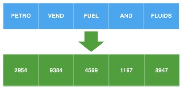
Why is hashing a useful trick?

In the video, Peter explained that a hash function takes an input, in your case a token, and outputs a hash value. For example, the input may be a string and the hash value may be an integer.

We’ve loaded a familiar python datatype, a dictionary called hash_dict, that makes this mapping concept a bit more explicit. In fact, python dictionaries ARE hash tables!

Print hash_dict in the IPython Shell to get a sense of how strings can be mapped to integers.

By explicitly stating how many possible outputs the hashing function may have, we limit the size of the objects that need to be processed. With these limits known, computation can be made more efficient and we can get results faster, even on large datasets.

Using the above information, answer the following:

Why is hashing a useful trick?

Instructions

~~Hashing isn’t useful unless you’re working with numbers.~~
~~Some problems are memory-bound and not easily parallelizable, but hashing parallelizes them.~~
Some problems are memory-bound and not easily parallelizable, and hashing enforces a fixed length computation instead of using a mutable datatype (like a dictionary). - Enforcing a fixed length can speed up calculations drastically, especially on large datasets!
~~Hashing enforces a mutable length computation instead of using a fixed length datatype, like a dictionary.~~

  
hash_dict = {'and': 780, 'fluids': 354, 'fuel': 895, 'petro': 354, 'vend': 785}

Implementing the hashing trick in scikit-learn

In this exercise you will check out the scikit-learn implementation of HashingVectorizer before adding it to your pipeline later.

As you saw in the video, HashingVectorizer acts just like CountVectorizer in that it can accept token_pattern and ngram_range parameters. The important difference is that it creates hash values from the text, so that we get all the computational advantages of hashing!

Instructions

Import HashingVectorizer from sklearn.feature_extraction.text.
Instantiate the HashingVectorizer as hashing_vec using the TOKENS_ALPHANUMERIC pattern.
Fit and transform hashing_vec using text_data. Save the result as hashed_text.
Hit submit to see some of the resulting hash values.

  
# Get text data: text_data
text_data = combine_text_columns(X_train)

# Create the token pattern: TOKENS_ALPHANUMERIC
TOKENS_ALPHANUMERIC = '[A-Za-z0-9]+(?=\\s+)' 

# Instantiate the HashingVectorizer: hashing_vec
hashing_vec = HashingVectorizer(token_pattern=TOKENS_ALPHANUMERIC)

# Fit and transform the Hashing Vectorizer
hashed_text = hashing_vec.fit_transform(text_data)

# Create DataFrame and print the head
hashed_df = pd.DataFrame(hashed_text.data)
print(hashed_df.head())

As you can see, some text is hashed to the same value, but as Peter mentioned in the video, this doesn’t neccessarily hurt performance.

Build the winning model

You have arrived! This is where all of your hard work pays off. It’s time to build the model that won DrivenData’s competition.

You’ve constructed a robust, powerful pipeline capable of processing training and testing data. Now that you understand the data and know all of the tools you need, you can essentially solve the whole problem in a relatively small number of lines of code. Wow!

All you need to do is add the HashingVectorizer step to the pipeline to replace the CountVectorizer step.

The parameters non_negative=True, norm=None, and binary=False make the HashingVectorizer perform similarly to the default settings on the CountVectorizer so you can just replace one with the other.

Instructions

Import HashingVectorizer from sklearn.feature_extraction.text.
Add a HashingVectorizer step to the pipeline.
- Name the step 'vectorizer'.
- Use the TOKENS_ALPHANUMERIC token pattern.
- Specify the ngram_range to be (1, 2)

  
# Instantiate the winning model pipeline: pl
pl = Pipeline([
    ('union', FeatureUnion(
        transformer_list=[
            ('numeric_features', Pipeline([
                ('selector', get_numeric_data),
                ('imputer', SimpleImputer())
            ])),
            ('text_features', Pipeline([
                ('selector', get_text_data),
                ('vectorizer', HashingVectorizer(token_pattern=TOKENS_ALPHANUMERIC,
                                                 alternate_sign=False, norm=None, binary=False,
                                                 ngram_range=(1, 2))),
                ('dim_red', SelectKBest(chi2, k=chi_k))
            ]))
        ]
    )),
    ('int', SparseInteractions(degree=2)),
    ('scale', MaxAbsScaler()),
    ('clf', OneVsRestClassifier(LogisticRegression()))
])

# fit the pipeline to our training data
pl.fit(X_train, y_train.values)

# print the score of our trained pipeline on our test set
log_loss_scorer = make_scorer(_multi_multi_log_loss)
print("Logloss score of trained pipeline: ", log_loss_scorer(pl, X_test, y_test.values))

Logloss score of trained pipeline:  3.654884613177857

Looks like the performance is about the same, but this is expected since the HashingVectorizer should work the same as the CountVectorizer. Try this pipeline out on the whole dataset on your local machine to see its full power!

What tactics got the winner the best score?

Now you’ve implemented the winning model from start to finish. If you want to use this model locally, this Jupyter notebook contains all the code you’ve worked so hard on. You can now take that code and build on it!

Let’s take a moment to reflect on why this model did so well. What tactics got the winner the best score?

Answer the question

The winner used a 500 layer deep convolutional neural network to master the budget data.
The winner used an ensemble of many models for classification, taking the best results as predictions.
The winner used skillful NLP, efficient computation, and simple but powerful stats tricks to master the budget data. - Often times simpler is better, and understanding the problem in depth leads to simpler solutions!

Next steps and the social impact of your work: Congratulations on finishing this course! I hope you enjoyed it and learned some useful tools to add to your data science toolbox. Your new skills have the ability to really make a difference. The volume of data is growing everywhere, not only in the tech industry. And with this growth in data comes opportunity: the opportunity to use your data science skills to make people’s lives better.
Can you do better?: One of our goals has been to demonstrate how flexible and powerful the Pipeline API is in scikit-learn. We’ve successively added small code changes that have had a big effect on our model. Now we want you to think about how you might improve things. Some areas to look at might be: Including stemming or stop-word removal in your natural language processing. Trying a different class of model like RandomForest, KNN or Naive Bayes. Doing further processing on the numeric columns and handling NaNs differently than the default Imputer. One of the benefits of scikit-learn is GridSearch (as you learned about in the supervised learning course). Check out the scikit-learn documentation to see how to perform grid search over every object in a Pipeline. You could even look around the scikit-learn docs and experiment with a new technique you haven’t used before. Feel free to sign up on DrivenData and experiment with some of these methods on the full dataset. Learning how these approaches effect real-world data can be a huge boost to your skills.
- You’ve seen the flexibility of the pipeline steps
- Quickly test ways of improving your submission
  - NLP: Stemming, stop-word removal
  - Model: RandomForest, k-NN, Naïve Bayes
  - Numeric Preprocessing: Imputation strategies
  - Optimization: Grid search over pipeline objects
  - Experiment with new scikit-learn techniques
- Work with the full dataset at DrivenData!
Hundreds of hours saved: The goal of building this model was to make an education non-profit more effective in helping school districts with their budgeting decisions. Having a model like the one we have built saves hundreds of hours a year in human time that was spent simply labeling line items. Now budget analysts can spend their time on the decisions that really matter.
- Make schools more efficient by improving their budgeting decisions
- Saves hundreds of hours each year that humans spent labeling line items
- Can spend more time on the decisions that really ma
DrivenData: Data Science to save the world: If you’re interested in other ways to use data science to have a social impact, we invite you to check out www-dot-drivendata-dot-org. We’ve always got competitions just like this running where you can look at new datasets, try interesting methods, learn from the community, and have an impact.
- Other ways to use data science to have a social impact at DrivenData
- Improve your data science skills while helping meaningful organizations thrive
- Win some cash prizes while you’re at it!

Certificate

Python, Machine Learning, Data Analysis, Data Science

This post is licensed under CC BY 4.0 by the author.

Introduction

Course Description

Imports

Saving data from DataCamp to a local csv

Exploring the Raw Data

Introducing the challenge

What category of problem is this?

What is the goal of the algorithm?

Exploring the data

Loading the data

Summarize the Data

Looking at the datatypes

Exploring datatypes in pandas

Encode the Labels as Categorical Variables

Counting Unique Labels

How do we measure success?

def compute_log_loss

Penalizing highly confident wrong answers

Computing log loss with Numpy

Creating a simple first model

It’s time to build a model

Setting up a train-test split in scikit-learn

Training a model

Making predictions

Use your model to predict values on holdout data

Writing out your results to a csv for submission

A very brief introduction to NLP

Tokenizating text

Testing your NLP credentials with n-grams

Representing text numerically

Combining text columns for tokenization

What’s in a token?

Improving your model

Pipelines, feature & text preprocessing

Instantiate pipeline

Preprocessing numeric features

Test features and feature union

Preprocessing text features

Multiple types of processing: FunctionTransformer

Multiple types of processing: FeatureUnion

Choosing a classification model

Using FunctionTransformer on the main dataset

Add a model to the pipeline

Try a different class of model

Can you adjust the model or parameters to improve accuracy?

Learning from the experts

Learning from the expert: processing

How many tokens?

Deciding what’s a word

N-gram range in scikit-learn

Learning from the expert: a stats trick

Which models of the data include interaction terms?

Implement interaction modeling in scikit-learn

Learning from the expert: the winning model

Why is hashing a useful trick?

Implementing the hashing trick in scikit-learn

Build the winning model

What tactics got the winner the best score?

Next steps and the social impact of your work

Certificate

Trending Tags

`def compute_log_loss`