Analysis of Stack Overflow Posting Trends

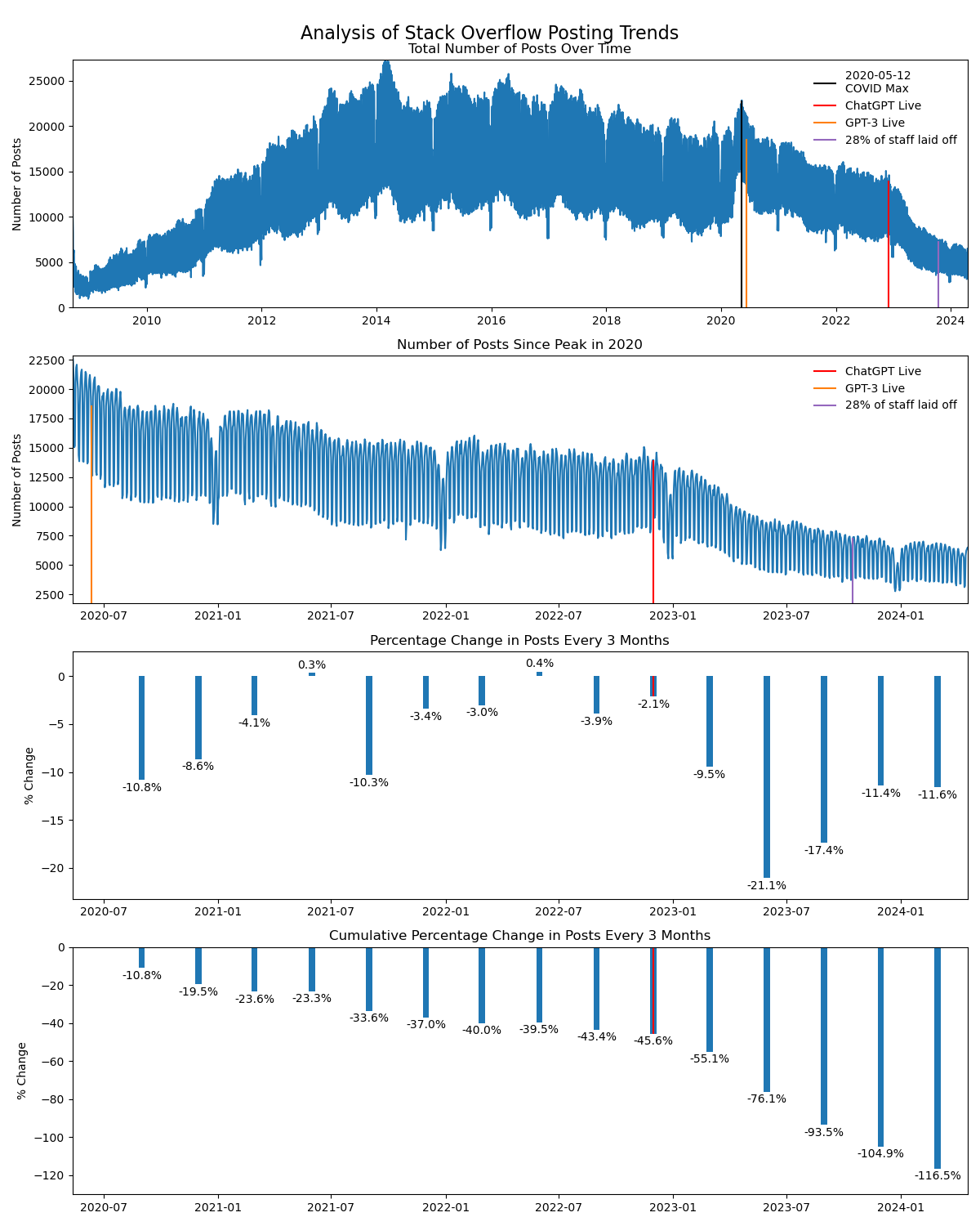
In this analysis, we explore the posting trends on Stack Overflow. We use Python and Pandas to analyze the data, focusing on the total number of posts over time, the number of posts since the peak in 2020, and the percentage change in posts every three months.

On the 12th of May, 2020, Stack Overflow experienced its highest activity since its previous peak on the 25th of February, 2014, with a total of 22,853 posts. However, a significant decrease in the number of posts has been observed since this peak. To analyze this trend, we employ the pct_change() function. This function calculates the percentage change between a current element and a preceding one. If the current element’s value is less than the preceding one, the percentage change will be negative.

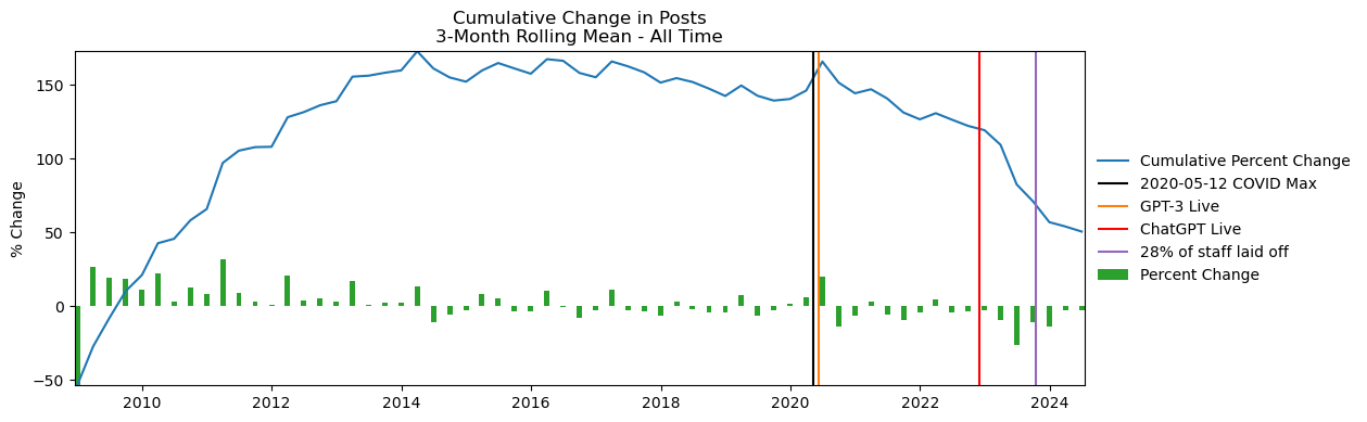
To track the overall trend, we use cumsum() on these values. This function adds up all the previous percent changes, including the negative ones. This can result in a cumulative percent change of less than -100%.

As of May 2024, we observe a decline of 118%. This doesn’t imply that the current value is below 0. Instead, it means that the cumulative sum of the percent changes from the start of our data to the current point is -118%. In other words, the number of posts has decreased by 118% compared to the sum of the individual changes over time.

This analysis provides valuable insights into the posting trends on Stack Overflow. It’s crucial to note that while we can observe the trends, further investigation would be needed to understand the underlying causes of these changes.

2024-05-31 is not included in the following plot as it is an incomplete period.

Stack Overflow Posting Trends Since 2020

Stack Overflow Cumulative Posting Trends For All Time

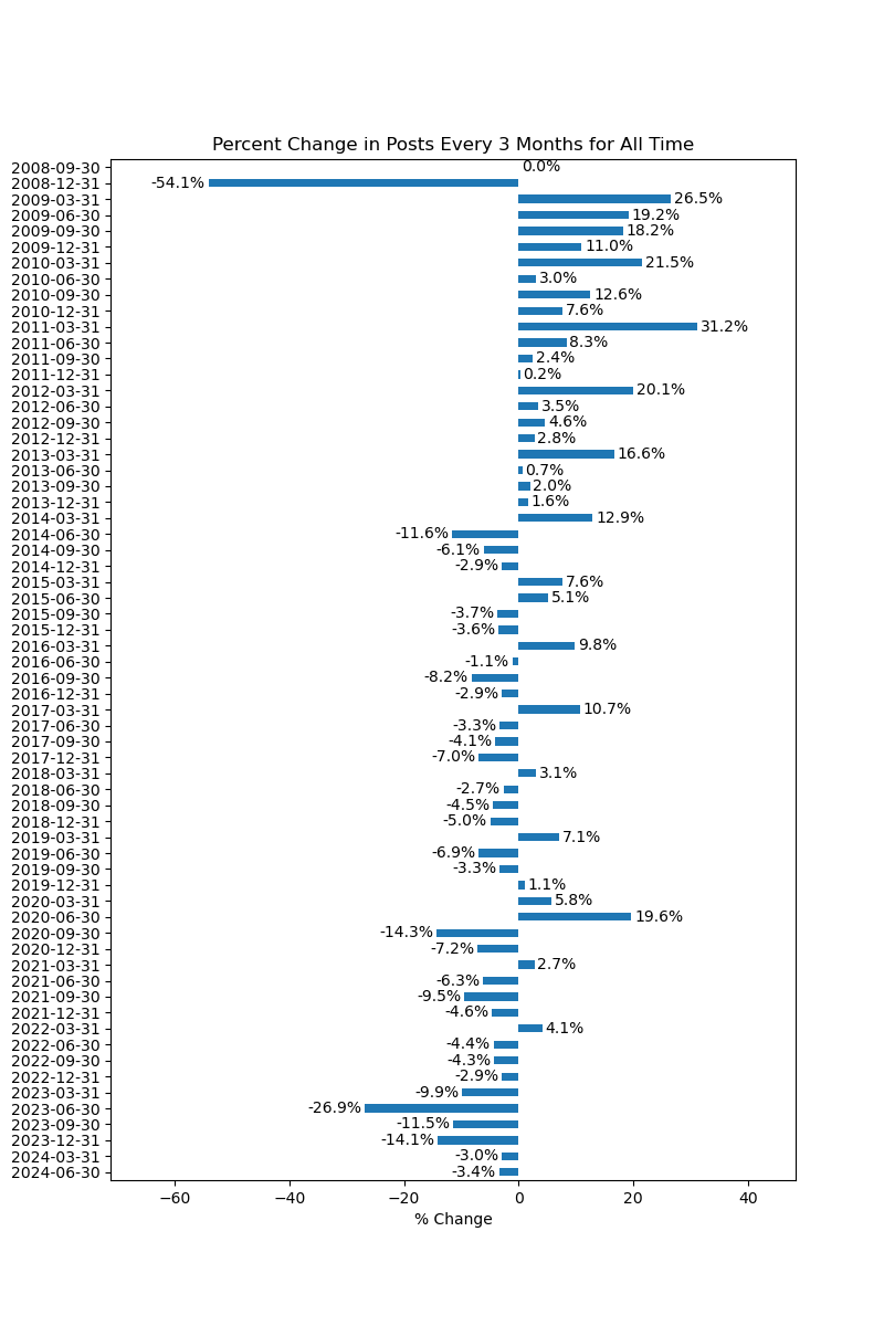
Percentage Change in Posts Every 3 Months for All Time

Cumulative Percentage Change in Posts Every 3 Months

Below is the cumulative percentage change in posts every three months since May 2020:

             all posts
2020-05-31         NaN
2020-08-31  -10.839550
2020-11-30  -19.483651
2021-02-28  -23.593446
2021-05-31  -23.263876
2021-08-31  -33.568631
2021-11-30  -36.951024
2022-02-28  -39.967492
2022-05-31  -39.528387
2022-08-31  -43.438464
2022-11-30  -45.571881
2023-02-28  -55.055765
2023-05-31  -76.122274
2023-08-31  -93.498322
2023-11-30 -104.921912
2024-02-29 -116.523075
2024-05-31 -118.265944

Percentage Change in Posts Every 3 Months

The following table shows the percent change in posts every 3 months:

            all posts
2020-05-31        NaN
2020-08-31 -10.839550
2020-11-30  -8.644101
2021-02-28  -4.109795
2021-05-31   0.329570
2021-08-31 -10.304755
2021-11-30  -3.382393
2022-02-28  -3.016468
2022-05-31   0.439105
2022-08-31  -3.910077
2022-11-30  -2.133418
2023-02-28  -9.483884
2023-05-31 -21.066510
2023-08-31 -17.376048
2023-11-30 -11.423590
2024-02-29 -11.601163
2024-05-31  -1.742869

Cumulative Percentage Change in Posts Every 3 Months for All Time

             all posts
2008-09-30         NaN
2008-12-31  -54.130519
2009-03-31  -27.649706
2009-06-30   -8.476289
2009-09-30    9.773043
2009-12-31   20.745324
2010-03-31   42.290162
2010-06-30   45.303434
2010-09-30   57.858498
2010-12-31   65.470041
2011-03-31   96.712762
2011-06-30  105.044830
2011-09-30  107.437054
2011-12-31  107.659922
2012-03-31  127.724477
2012-06-30  131.178286
2012-09-30  135.827747
2012-12-31  138.583285
2013-03-31  155.216138
2013-06-30  155.880021
2013-09-30  157.870281
2013-12-31  159.481414
2014-03-31  172.417210
2014-06-30  160.788770
2014-09-30  154.675661
2014-12-31  151.803114
2015-03-31  159.389766
2015-06-30  164.460737
2015-09-30  160.776255
2015-12-31  157.204343
2016-03-31  167.053985
2016-06-30  165.974997
2016-09-30  157.748778
2016-12-31  154.801111
2017-03-31  165.533354
2017-06-30  162.235831
2017-09-30  158.129740
2017-12-31  151.178991
2018-03-31  154.229334
2018-06-30  151.572721
2018-09-30  147.096148
2018-12-31  142.122814
2019-03-31  149.214841
2019-06-30  142.282671
2019-09-30  138.991455
2019-12-31  140.078815
2020-03-31  145.833111
2020-06-30  165.479189
2020-09-30  151.146378
2020-12-31  143.945442
2021-03-31  146.679697
2021-06-30  140.421901
2021-09-30  130.896650
2021-12-31  126.283470
2022-03-31  130.425047
2022-06-30  126.046113
2022-09-30  121.793145
2022-12-31  118.908208
2023-03-31  109.001864
2023-06-30   82.149043
2023-09-30   70.638653
2023-12-31   56.550648
2024-03-31   53.595146
2024-06-30   50.183799

Code to Generate the Analysis

import pandas as pd
import matplotlib.pyplot as plt
from datetime import datetime, date

# Load the data from a CSV file, parsing 'date' column as dates and setting it as index
df = pd.read_csv('data/site_data/posts_2008-Sep-15_2024-Apr-18.csv', parse_dates=['date'],
                 usecols=['date', 'all posts'], index_col='date')

# Filter the data to include only entries from 2020 onwards
df_2020 = df.loc['2020':]

# Find the date with the most posts in the filtered data
max_2020 = pd.Timestamp(df_2020.idxmax().values[0]).date()

# Adjust df_2020 to show only data from the date with most posts onwards
df_2020 = df_2020.loc[max_2020:]

# Resample the data to 3-month periods and calculate the mean for each period
df_resampled = df_2020.resample('3ME').mean()

# Calculate the percent change for each period
df_percent_change = df_resampled.pct_change().mul(100)

# Set the index to be the date component only
df_percent_change.index = df_percent_change.index.date

# Calculate the cumulative percent change and convert it to percentage
df_cumulative_percent_change = df_percent_change.cumsum()

# Create a subplot with 3 rows
fig, (ax0, ax1, ax2, ax3) = plt.subplots(nrows=4, figsize=(12, 15), tight_layout=True)

# Plot the entire data on the first subplot
ax0.plot(df, label='')
ymin, ymax = ax0.get_ylim()
ax0.vlines(x=max_2020, ymin=ymin, ymax=df_2020.max(), label=f'{max_2020}\nCOVID Max', colors='k')

# Plot the filtered data on the second subplot
ax1.plot('date', 'all posts', data=df_2020.reset_index(), label='')

# Plot the cumulative percent change as a bar chart on the third subplot
ax2.bar(x='index', height='all posts', width=10, data=df_percent_change.reset_index(), label='')

# Add labels to the bars on the third subplot
ax2.bar_label(ax2.containers[0], padding=2, fmt='%.1f%%')

# Bar Plot the cumulative percent change as a line chart on the fourth subplot
ax3.bar(x='index', height='all posts', width=10, data=df_cumulative_percent_change.reset_index(), label='')

# Add labels to the bars on the fourth subplot
ax3.bar_label(ax3.containers[0], padding=2, fmt='%.1f%%')

# Define the date when ChatGPT went live
chatGPT_day = datetime.strptime('2022-11-30', '%Y-%m-%d')

# Add a vertical line on the third subplot at the date when ChatGPT went live
ax2.vlines(x=chatGPT_day, ymin=df_percent_change.loc[date(2022, 11, 30), 'all posts'],
           ymax=0, label='ChatGPT Live', colors='r')

# Add a vertical line on the fourth subplot at the date when ChatGPT went live
ax3.vlines(x=chatGPT_day, ymin=df_cumulative_percent_change.loc[date(2022, 11, 30), 'all posts'],
           ymax=0, label='ChatGPT Live', colors='r')

# Add a vertical line on the first and second subplots at the date when ChatGPT went live
for ax in [ax0, ax1]:
    ymin, _ = ax.get_ylim()
    ymax = df.loc[chatGPT_day, 'all posts']
    ax.vlines(x=chatGPT_day, ymin=ymin, ymax=ymax, label='ChatGPT Live', colors='r')
    # add a line for the date when GPT-3 went live
    ax.vlines(x=datetime.strptime('2020-06-11', '%Y-%m-%d'), ymin=ymin,
              ymax=df.loc['2020-06-11', 'all posts'], label='GPT-3 Live', colors='tab:orange')
    # add a line for the date of stack overflow's 2023-10-16 layoffs
    ax.vlines(x=datetime.strptime('2023-10-16', '%Y-%m-%d'), ymin=ymin,
              ymax=df.loc['2023-10-16', 'all posts'], label='28% of staff laid off', colors='tab:purple')
    ax.legend(frameon=False)

# Set margins for the first and second subplots
ax0.margins(x=0, y=0)
ax1.margins(y=0)
ax2.margins(y=0.1)
ax3.margins(y=0.1)

# Set limits for the x and y axes of the subplots
ax0.set_ylim(bottom=0)
ax0.set_xlim(left=df.index.min(), right=df.index.max())
ax1.set_xlim(left=df_2020.index.min(), right=df_2020.index.max())
ax2.set_xlim(left=df_2020.index.min(), right=df_2020.index.max())
ax3.set_xlim(left=df_2020.index.min(), right=df_2020.index.max())

# Set titles and y-labels for the subplots
ax0.set(title='Total Number of Posts Over Time', ylabel='Number of Posts')
ax1.set(title='Number of Posts Since Peak in 2020', ylabel='Number of Posts')
ax2.set(title='Percentage Change in Posts Every 3 Months', ylabel='% Change')
ax3.set(title='Cumulative Percentage Change in Posts Every 3 Months', ylabel='% Change')

# Add a suptitle to the figure
_ = fig.suptitle('Analysis of Stack Overflow Posting Trends', fontsize=16)

# Save the plot as a PNG file
plt.savefig('2024-04-19-decline-of-stack-overflow-posting.png')

# Display the plot
plt.show()