Introduction
1
2
3
4
5
6
| import pandas as pd
import matplotlib.pyplot as plt
import numpy as np
from numpy import NaN
from glob import glob
import re
|
1
2
3
| pd.set_option('display.max_columns', 200)
pd.set_option('display.max_rows', 300)
pd.set_option('display.expand_frame_repr', True)
|
Course Description
Pandas DataFrames are the most widely used in-memory representation of complex data collections within Python. Whether in finance, scientific fields, or data science, a familiarity with Pandas is essential. This course teaches you to work with real-world data sets containing both string and numeric data, often structured around time series. You will learn powerful analysis, selection, and visualization techniques in this course.
Synopsis
Data Ingestion & Inspection
- Data loaded into a DataFrame from a CSV file.
- First few rows of the DataFrame displayed using
head(). - Columns renamed to be more descriptive.
- Data types of each column inspected using
dtypes. - Rows with missing data identified using
isna().any(). - Summary statistics generated with
describe().
Exploratory Data Analysis
- Histograms created to visualize distributions of numerical columns.
- Box plots generated to identify outliers.
- Scatter plots used to examine relationships between variables.
- Grouping operations performed using
groupby(). - Pivot tables created for summary statistics.
Time Series in pandas
- Date and time information set as the index of the DataFrame.
- Data resampled to different frequencies (e.g., daily, monthly) using
resample(). - Rolling averages calculated to smooth time series data.
- Time series plotted to visualize trends over time.
Case Study - Sunlight in Austin
- Data filtered to specific time periods.
- Specific conditions (e.g., overcast days) identified using string operations.
- Daily maximum temperatures calculated for filtered data.
- Cumulative distribution function (CDF) constructed for specific subsets of data.
- Findings summarized and visualized with appropriate plots.
Data Files
Data ingestion & inspection
In this chapter, you will be introduced to Panda’s DataFrames. You will use Pandas to import and inspect a variety of datasets, ranging from population data obtained from The World Bank to monthly stock data obtained via Yahoo! Finance. You will also practice building DataFrames from scratch, and become familiar with Pandas’ intrinsic data visualization capabilities.
Review pandas DataFrames
- Example: DataFrame of Apple Stock data
1
2
| AAPL = pd.read_csv(r'DataCamp-master/11-pandas-foundations/_datasets/AAPL.csv',
index_col='Date', parse_dates=True)
|
| Open | High | Low | Close | Adj Close | Volume |
|---|
| Date | | | | | | |
|---|
| 1980-12-12 | 0.513393 | 0.515625 | 0.513393 | 0.513393 | 0.023106 | 117258400.0 |
|---|
| 1980-12-15 | 0.488839 | 0.488839 | 0.486607 | 0.486607 | 0.021900 | 43971200.0 |
|---|
| 1980-12-16 | 0.453125 | 0.453125 | 0.450893 | 0.450893 | 0.020293 | 26432000.0 |
|---|
| 1980-12-17 | 0.462054 | 0.464286 | 0.462054 | 0.462054 | 0.020795 | 21610400.0 |
|---|
| 1980-12-18 | 0.475446 | 0.477679 | 0.475446 | 0.475446 | 0.021398 | 18362400.0 |
|---|
- The rows are labeled by a special data structure called an Index.
- Indexes in Pandas are tailored lists of labels that permit fast look-up and some powerful relational operations.
- The index labels in the AAPL DataFrame are dates in reverse chronological order.
- Labeled rows & columns improves the clarity and intuition of many data analysis tasks.
1
| pandas.core.frame.DataFrame
|
1
| Index(['Open', 'High', 'Low', 'Close', 'Adj Close', 'Volume'], dtype='object')
|
1
| pandas.core.indexes.base.Index
|
1
2
3
4
5
6
7
8
| DatetimeIndex(['1980-12-12', '1980-12-15', '1980-12-16', '1980-12-17',
'1980-12-18', '1980-12-19', '1980-12-22', '1980-12-23',
'1980-12-24', '1980-12-26',
...
'2019-01-10', '2019-01-11', '2019-01-14', '2019-01-15',
'2019-01-16', '2019-01-17', '2019-01-18', '2019-01-22',
'2019-01-23', '2019-01-24'],
dtype='datetime64[ns]', name='Date', length=9611, freq=None)
|
1
| pandas.core.indexes.datetimes.DatetimeIndex
|
- DataFrames can be sliced like NumPy arrays or Python lists using colons to specify the start, end and stride of a slice.
1
2
| # Start of the DataFrame to the 5th row, inclusive of all columns
AAPL.iloc[:5,:]
|
| Open | High | Low | Close | Adj Close | Volume |
|---|
| Date | | | | | | |
|---|
| 1980-12-12 | 0.513393 | 0.515625 | 0.513393 | 0.513393 | 0.023106 | 117258400.0 |
|---|
| 1980-12-15 | 0.488839 | 0.488839 | 0.486607 | 0.486607 | 0.021900 | 43971200.0 |
|---|
| 1980-12-16 | 0.453125 | 0.453125 | 0.450893 | 0.450893 | 0.020293 | 26432000.0 |
|---|
| 1980-12-17 | 0.462054 | 0.464286 | 0.462054 | 0.462054 | 0.020795 | 21610400.0 |
|---|
| 1980-12-18 | 0.475446 | 0.477679 | 0.475446 | 0.475446 | 0.021398 | 18362400.0 |
|---|
1
2
| # Start at the 5th last row to the end of the DataFrame using a negative index
AAPL.iloc[-5:,:]
|
| Open | High | Low | Close | Adj Close | Volume |
|---|
| Date | | | | | | |
|---|
| 2019-01-17 | 154.199997 | 157.660004 | 153.259995 | 155.860001 | 155.860001 | 29821200.0 |
|---|
| 2019-01-18 | 157.500000 | 157.880005 | 155.979996 | 156.820007 | 156.820007 | 33751000.0 |
|---|
| 2019-01-22 | 156.410004 | 156.729996 | 152.619995 | 153.300003 | 153.300003 | 30394000.0 |
|---|
| 2019-01-23 | 154.149994 | 155.139999 | 151.699997 | 153.919998 | 153.919998 | 23130600.0 |
|---|
| 2019-01-24 | 154.110001 | 154.479996 | 151.740005 | 152.699997 | 152.699997 | 25421800.0 |
|---|
| Open | High | Low | Close | Adj Close | Volume |
|---|
| Date | | | | | | |
|---|
| 1980-12-12 | 0.513393 | 0.515625 | 0.513393 | 0.513393 | 0.023106 | 117258400.0 |
|---|
| 1980-12-15 | 0.488839 | 0.488839 | 0.486607 | 0.486607 | 0.021900 | 43971200.0 |
|---|
| 1980-12-16 | 0.453125 | 0.453125 | 0.450893 | 0.450893 | 0.020293 | 26432000.0 |
|---|
| 1980-12-17 | 0.462054 | 0.464286 | 0.462054 | 0.462054 | 0.020795 | 21610400.0 |
|---|
| 1980-12-18 | 0.475446 | 0.477679 | 0.475446 | 0.475446 | 0.021398 | 18362400.0 |
|---|
| Open | High | Low | Close | Adj Close | Volume |
|---|
| Date | | | | | | |
|---|
| 2019-01-17 | 154.199997 | 157.660004 | 153.259995 | 155.860001 | 155.860001 | 29821200.0 |
|---|
| 2019-01-18 | 157.500000 | 157.880005 | 155.979996 | 156.820007 | 156.820007 | 33751000.0 |
|---|
| 2019-01-22 | 156.410004 | 156.729996 | 152.619995 | 153.300003 | 153.300003 | 30394000.0 |
|---|
| 2019-01-23 | 154.149994 | 155.139999 | 151.699997 | 153.919998 | 153.919998 | 23130600.0 |
|---|
| 2019-01-24 | 154.110001 | 154.479996 | 151.740005 | 152.699997 | 152.699997 | 25421800.0 |
|---|
1
2
3
4
5
6
7
8
9
10
11
12
13
| <class 'pandas.core.frame.DataFrame'>
DatetimeIndex: 9611 entries, 1980-12-12 to 2019-01-24
Data columns (total 6 columns):
# Column Non-Null Count Dtype
--- ------ -------------- -----
0 Open 9610 non-null float64
1 High 9610 non-null float64
2 Low 9610 non-null float64
3 Close 9610 non-null float64
4 Adj Close 9610 non-null float64
5 Volume 9610 non-null float64
dtypes: float64(6)
memory usage: 525.6 KB
|
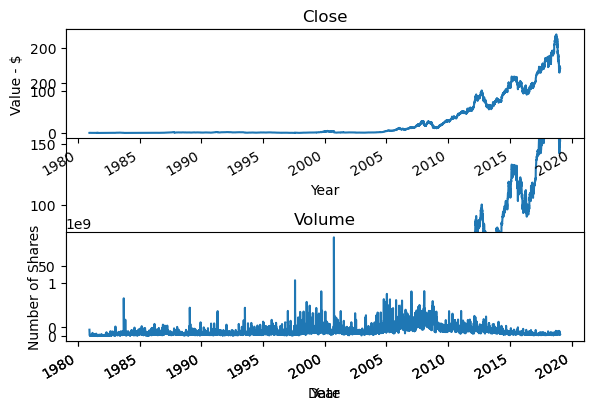
1
2
3
4
5
6
7
8
9
10
11
12
13
14
15
16
17
18
19
20
21
22
23
| AAPL.Close.plot(kind='line')
# Add first subplot
plt.subplot(2, 1, 1)
AAPL.Close.plot(kind='line')
# Add title and specify axis labels
plt.title('Close')
plt.ylabel('Value - $')
plt.xlabel('Year')
# Add second subplot
plt.subplot(2, 1, 2)
AAPL.Volume.plot(kind='line')
# Add title and specify axis labels
plt.title('Volume')
plt.ylabel('Number of Shares')
plt.xlabel('Year')
# Display the plots
plt.tight_layout()
plt.show()
|
Broadcasting
- Assigning scalar value to column slice broadcasts value to each row
1
| AAPL.iloc[::3, -1] = np.nan # every 3rd row of Volume is now NaN
|
| Open | High | Low | Close | Adj Close | Volume |
|---|
| Date | | | | | | |
|---|
| 1980-12-12 | 0.513393 | 0.515625 | 0.513393 | 0.513393 | 0.023106 | NaN |
|---|
| 1980-12-15 | 0.488839 | 0.488839 | 0.486607 | 0.486607 | 0.021900 | 43971200.0 |
|---|
| 1980-12-16 | 0.453125 | 0.453125 | 0.450893 | 0.450893 | 0.020293 | 26432000.0 |
|---|
| 1980-12-17 | 0.462054 | 0.464286 | 0.462054 | 0.462054 | 0.020795 | NaN |
|---|
| 1980-12-18 | 0.475446 | 0.477679 | 0.475446 | 0.475446 | 0.021398 | 18362400.0 |
|---|
| 1980-12-19 | 0.504464 | 0.506696 | 0.504464 | 0.504464 | 0.022704 | 12157600.0 |
|---|
| 1980-12-22 | 0.529018 | 0.531250 | 0.529018 | 0.529018 | 0.023809 | NaN |
|---|
1
2
3
4
5
6
7
8
9
10
11
12
13
| <class 'pandas.core.frame.DataFrame'>
DatetimeIndex: 9611 entries, 1980-12-12 to 2019-01-24
Data columns (total 6 columns):
# Column Non-Null Count Dtype
--- ------ -------------- -----
0 Open 9610 non-null float64
1 High 9610 non-null float64
2 Low 9610 non-null float64
3 Close 9610 non-null float64
4 Adj Close 9610 non-null float64
5 Volume 6407 non-null float64
dtypes: float64(6)
memory usage: 525.6 KB
|
- Note Volume now has few non-null numbers
Series
1
| pandas.core.series.Series
|
1
2
3
4
5
6
7
| Date
1980-12-12 0.513393
1980-12-15 0.486607
1980-12-16 0.450893
1980-12-17 0.462054
1980-12-18 0.475446
Name: Low, dtype: float64
|
1
| array([0.513393, 0.486607, 0.450893, 0.462054, 0.475446])
|
- A Pandas Series, then, is a 1D labeled NumPy array and a DataFrame is a 2D labeled array whose columns as Series
Exercises
Inspecting your data
You can use the DataFrame methods .head() and .tail() to view the first few and last few rows of a DataFrame. In this exercise, we have imported pandas as pd and loaded population data from 1960 to 2014 as a DataFrame df. This dataset was obtained from the World Bank.
Your job is to use df.head() and df.tail() to verify that the first and last rows match a file on disk. In later exercises, you will see how to extract values from DataFrames with indexing, but for now, manually copy/paste or type values into assignment statements where needed. Select the correct answer for the first and last values in the 'Year' and 'Total Population' columns.
Instructions
Possible Answers
- First: 1980, 26183676.0; Last: 2000, 35.
- First: 1960, 92495902.0; Last: 2014, 15245855.0.
- First: 40.472, 2001; Last: 44.5, 1880.
- First: CSS, 104170.0; Last: USA, 95.203.
1
| wb_df = pd.read_csv(r'DataCamp-master/11-pandas-foundations/_datasets/world_ind_pop_data.csv')
|
| CountryName | CountryCode | Year | Total Population | Urban population (% of total) |
|---|
| 0 | Arab World | ARB | 1960 | 9.249590e+07 | 31.285384 |
|---|
| 1 | Caribbean small states | CSS | 1960 | 4.190810e+06 | 31.597490 |
|---|
| 2 | Central Europe and the Baltics | CEB | 1960 | 9.140158e+07 | 44.507921 |
|---|
| 3 | East Asia & Pacific (all income levels) | EAS | 1960 | 1.042475e+09 | 22.471132 |
|---|
| 4 | East Asia & Pacific (developing only) | EAP | 1960 | 8.964930e+08 | 16.917679 |
|---|
| CountryName | CountryCode | Year | Total Population | Urban population (% of total) |
|---|
| 13369 | Virgin Islands (U.S.) | VIR | 2014 | 104170.0 | 95.203 |
|---|
| 13370 | West Bank and Gaza | WBG | 2014 | 4294682.0 | 75.026 |
|---|
| 13371 | Yemen, Rep. | YEM | 2014 | 26183676.0 | 34.027 |
|---|
| 13372 | Zambia | ZMB | 2014 | 15721343.0 | 40.472 |
|---|
| 13373 | Zimbabwe | ZWE | 2014 | 15245855.0 | 32.501 |
|---|
DataFrame data types
Pandas is aware of the data types in the columns of your DataFrame. It is also aware of null and NaN (‘Not-a-Number’) types which often indicate missing data. In this exercise, we have imported pandas as pd and read in the world population data which contains some NaN values, a value often used as a place-holder for missing or otherwise invalid data entries. Your job is to use df.info() to determine information about the total count of non-null entries and infer the total count of 'null' entries, which likely indicates missing data. Select the best description of this data set from the following:
Instructions
Possible Answers
- The data is all of type float64 and none of it is missing.
- The data is of mixed type, and 9914 of it is missing.
- The data is of mixed type, and 3460 float64s are missing.
- The data is all of type float64, and 3460 float64s are missing.
1
2
3
4
5
6
7
8
9
10
| <class 'pandas.core.frame.DataFrame'>
RangeIndex: 13374 entries, 0 to 13373
Data columns (total 5 columns):
CountryName 13374 non-null object
CountryCode 13374 non-null object
Year 13374 non-null int64
Total Population 9914 non-null float64
Urban population (% of total) 13374 non-null float64
dtypes: float64(2), int64(1), object(2)
memory usage: 522.5+ KB
|
1
2
3
4
5
6
7
8
9
10
11
12
| <class 'pandas.core.frame.DataFrame'>
RangeIndex: 13374 entries, 0 to 13373
Data columns (total 5 columns):
# Column Non-Null Count Dtype
--- ------ -------------- -----
0 CountryName 13374 non-null object
1 CountryCode 13374 non-null object
2 Year 13374 non-null int64
3 Total Population 13374 non-null float64
4 Urban population (% of total) 13374 non-null float64
dtypes: float64(2), int64(1), object(2)
memory usage: 522.6+ KB
|
NumPy and pandas working together
Pandas depends upon and interoperates with NumPy, the Python library for fast numeric array computations. For example, you can use the DataFrame attribute .values to represent a DataFrame df as a NumPy array. You can also pass pandas data structures to NumPy methods. In this exercise, we have imported pandas as pd and loaded world population data every 10 years since 1960 into the DataFrame df. This dataset was derived from the one used in the previous exercise.
Your job is to extract the values and store them in an array using the attribute .values. You’ll then use those values as input into the NumPy np.log10() method to compute the base 10 logarithm of the population values. Finally, you will pass the entire pandas DataFrame into the same NumPy np.log10() method and compare the results.
Instructions
- Import
numpy using the standard alias np. - Assign the numerical values in the DataFrame
df to an array np_vals using the attribute values. - Pass
np_vals into the NumPy method log10() and store the results in np_vals_log10. - Pass the entire
df DataFrame into the NumPy method log10() and store the results in df_log10. - Inspect the output of the
print() code to see the type() of the variables that you created.
1
| pop_df = pd.read_csv(r'DataCamp-master/11-pandas-foundations/_datasets/world_population.csv')
|
1
2
3
4
5
6
7
8
9
| <class 'pandas.core.frame.DataFrame'>
RangeIndex: 6 entries, 0 to 5
Data columns (total 2 columns):
# Column Non-Null Count Dtype
--- ------ -------------- -----
0 Date 6 non-null int64
1 Total Population 6 non-null int64
dtypes: int64(2)
memory usage: 228.0 bytes
|
1
2
| # Create array of DataFrame values: np_vals
np_vals = pop_df.values
|
1
2
3
4
5
6
| array([[ 1960, 3034970564],
[ 1970, 3684822701],
[ 1980, 4436590356],
[ 1990, 5282715991],
[ 2000, 6115974486],
[ 2010, 6924282937]], dtype=int64)
|
1
2
| # Create new array of base 10 logarithm values: np_vals_log10
np_vals_log10 = np.log10(np_vals)
|
1
2
3
4
5
6
| array([[3.29225607, 9.48215448],
[3.29446623, 9.5664166 ],
[3.29666519, 9.64704933],
[3.29885308, 9.72285726],
[3.30103 , 9.78646566],
[3.30319606, 9.84037481]])
|
1
2
| # Create array of new DataFrame by passing df to np.log10(): df_log10
pop_df_log10 = np.log10(pop_df)
|
| Date | Total Population |
|---|
| 0 | 3.292256 | 9.482154 |
|---|
| 1 | 3.294466 | 9.566417 |
|---|
| 2 | 3.296665 | 9.647049 |
|---|
| 3 | 3.298853 | 9.722857 |
|---|
| 4 | 3.301030 | 9.786466 |
|---|
| 5 | 3.303196 | 9.840375 |
|---|
1
2
| # Print original and new data containers
[print(x, 'has type', type(eval(x))) for x in ['np_vals', 'np_vals_log10', 'pop_df', 'pop_df_log10']]
|
1
2
3
4
5
6
7
8
9
10
| np_vals has type <class 'numpy.ndarray'>
np_vals_log10 has type <class 'numpy.ndarray'>
pop_df has type <class 'pandas.core.frame.DataFrame'>
pop_df_log10 has type <class 'pandas.core.frame.DataFrame'>
[None, None, None, None]
|
As a data scientist, you’ll frequently interact with NumPy arrays, pandas Series, and pandas DataFrames, and you’ll leverage a variety of NumPy and pandas methods to perform your desired computations. Understanding how NumPy and pandas work together will prove to be very useful.
Building DataFrames from Scratch
- DataFrames read in from CSV
- DataFrames from dict (1)
1
2
3
4
| data = {'weekday': ['Sun', 'Sun', 'Mon', 'Mon'],
'city': ['Austin', 'Dallas', 'Austin', 'Dallas'],
'visitors': [139, 237, 326, 456],
'signups': [7, 12, 3, 5]}
|
1
| users = pd.DataFrame(data)
|
| weekday | city | visitors | signups |
|---|
| 0 | Sun | Austin | 139 | 7 |
|---|
| 1 | Sun | Dallas | 237 | 12 |
|---|
| 2 | Mon | Austin | 326 | 3 |
|---|
| 3 | Mon | Dallas | 456 | 5 |
|---|
1
2
3
4
5
6
7
8
9
10
| cities = ['Austin', 'Dallas', 'Austin', 'Dallas']
signups = [7, 12, 3, 5]
weekdays = ['Sun', 'Sun', 'Mon', 'Mon']
visitors = [139, 237, 326, 456]
list_labels = ['city', 'signups', 'visitors', 'weekday']
list_cols = [cities, signups, visitors, weekdays] # list of lists
zipped = list(zip(list_labels, list_cols)) # tuples
zipped
|
1
2
3
4
| [('city', ['Austin', 'Dallas', 'Austin', 'Dallas']),
('signups', [7, 12, 3, 5]),
('visitors', [139, 237, 326, 456]),
('weekday', ['Sun', 'Sun', 'Mon', 'Mon'])]
|
1
| users2 = pd.DataFrame(data2)
|
| city | signups | visitors | weekday |
|---|
| 0 | Austin | 7 | 139 | Sun |
|---|
| 1 | Dallas | 12 | 237 | Sun |
|---|
| 2 | Austin | 3 | 326 | Mon |
|---|
| 3 | Dallas | 5 | 456 | Mon |
|---|
Broadcasting
- Saves time by generating long lists, arrays or columns without loops
1
| users['fees'] = 0 # Broadcasts value to entire column
|
| weekday | city | visitors | signups | fees |
|---|
| 0 | Sun | Austin | 139 | 7 | 0 |
|---|
| 1 | Sun | Dallas | 237 | 12 | 0 |
|---|
| 2 | Mon | Austin | 326 | 3 | 0 |
|---|
| 3 | Mon | Dallas | 456 | 5 | 0 |
|---|
Broadcasting with a dict
1
| heights = [59.0, 65.2, 62.9, 65.4, 63.7, 65.7, 64.1]
|
1
| data = {'height': heights, 'sex': 'M'} # M is broadcast to the entire column
|
1
| results = pd.DataFrame(data)
|
| height | sex |
|---|
| 0 | 59.0 | M |
|---|
| 1 | 65.2 | M |
|---|
| 2 | 62.9 | M |
|---|
| 3 | 65.4 | M |
|---|
| 4 | 63.7 | M |
|---|
| 5 | 65.7 | M |
|---|
| 6 | 64.1 | M |
|---|
Index and columns
- We can assign list of strings to the attributes columns and index as long as they are of suitable length.
1
| results.columns = ['height (in)', 'sex']
|
1
| results.index = ['A', 'B', 'C', 'D', 'E', 'F', 'G']
|
| height (in) | sex |
|---|
| A | 59.0 | M |
|---|
| B | 65.2 | M |
|---|
| C | 62.9 | M |
|---|
| D | 65.4 | M |
|---|
| E | 63.7 | M |
|---|
| F | 65.7 | M |
|---|
| G | 64.1 | M |
|---|
Exercises
Zip lists to build a DataFrame
In this exercise, you’re going to make a pandas DataFrame of the top three countries to win gold medals since 1896 by first building a dictionary. list_keys contains the column names 'Country' and 'Total'. list_values contains the full names of each country and the number of gold medals awarded. The values have been taken from Wikipedia.
Your job is to use these lists to construct a list of tuples, use the list of tuples to construct a dictionary, and then use that dictionary to construct a DataFrame. In doing so, you’ll make use of the list(), zip(), dict() and pd.DataFrame() functions. Pandas has already been imported as pd.
Note: The zip() function in Python 3 and above returns a special zip object, which is essentially a generator. To convert this zip object into a list, you’ll need to use list(). You can learn more about the zip() function as well as generators in Python Data Science Toolbox (Part 2).
Instructions
- Zip the 2 lists
list_keys and list_values together into one list of (key, value) tuples. Be sure to convert the zip object into a list, and store the result in zipped. - Inspect the contents of
zipped using print(). This has been done for you. - Construct a dictionary using
zipped. Store the result as data. - Construct a DataFrame using the dictionary. Store the result as
df.
1
2
| list_keys = ['Country', 'Total']
list_values = [['United States', 'Soviet Union', 'United Kingdom'], [1118, 473, 273]]
|
1
2
| zipped = list(zip(list_keys, list_values)) # tuples
zipped
|
1
2
| [('Country', ['United States', 'Soviet Union', 'United Kingdom']),
('Total', [1118, 473, 273])]
|
1
2
| {'Country': ['United States', 'Soviet Union', 'United Kingdom'],
'Total': [1118, 473, 273]}
|
1
| data_df = pd.DataFrame.from_dict(data)
|
| Country | Total |
|---|
| 0 | United States | 1118 |
|---|
| 1 | Soviet Union | 473 |
|---|
| 2 | United Kingdom | 273 |
|---|
Labeling your data
You can use the DataFrame attribute df.columns to view and assign new string labels to columns in a pandas DataFrame.
In this exercise, we have imported pandas as pd and defined a DataFrame df containing top Billboard hits from the 1980s (from Wikipedia). Each row has the year, artist, song name and the number of weeks at the top. However, this DataFrame has the column labels a, b, c, d. Your job is to use the df.columns attribute to re-assign descriptive column labels.
Instructions
- Create a list of new column labels with
'year', 'artist', 'song', 'chart weeks', and assign it to list_labels. - Assign your list of labels to
df.columns.
1
2
3
4
5
6
7
| billboard_values = np.array([['1980', 'Blondie', 'Call Me', '6'],
['1981', 'Chistorpher Cross', 'Arthurs Theme', '3'],
['1982', 'Joan Jett', 'I Love Rock and Roll', '7']]).transpose()
billboard_keys = ['a', 'b', 'c', 'd']
billboard_zipped = list(zip(billboard_keys, billboard_values))
billboard_zipped
|
1
2
3
4
5
| [('a', array(['1980', '1981', '1982'], dtype='<U20')),
('b', array(['Blondie', 'Chistorpher Cross', 'Joan Jett'], dtype='<U20')),
('c',
array(['Call Me', 'Arthurs Theme', 'I Love Rock and Roll'], dtype='<U20')),
('d', array(['6', '3', '7'], dtype='<U20'))]
|
1
| billboard_dict = dict(billboard_zipped)
|
1
2
3
4
| {'a': array(['1980', '1981', '1982'], dtype='<U20'),
'b': array(['Blondie', 'Chistorpher Cross', 'Joan Jett'], dtype='<U20'),
'c': array(['Call Me', 'Arthurs Theme', 'I Love Rock and Roll'], dtype='<U20'),
'd': array(['6', '3', '7'], dtype='<U20')}
|
1
| billboard = pd.DataFrame.from_dict(billboard_dict)
|
| a | b | c | d |
|---|
| 0 | 1980 | Blondie | Call Me | 6 |
|---|
| 1 | 1981 | Chistorpher Cross | Arthurs Theme | 3 |
|---|
| 2 | 1982 | Joan Jett | I Love Rock and Roll | 7 |
|---|
1
2
| # Build a list of labels: list_labels
list_labels = ['year', 'artist', 'song', 'chart weeks']
|
1
2
| # Assign the list of labels to the columns attribute: df.columns
billboard.columns = list_labels
|
| year | artist | song | chart weeks |
|---|
| 0 | 1980 | Blondie | Call Me | 6 |
|---|
| 1 | 1981 | Chistorpher Cross | Arthurs Theme | 3 |
|---|
| 2 | 1982 | Joan Jett | I Love Rock and Roll | 7 |
|---|
Building DataFrames with broadcasting
You can implicitly use ‘broadcasting’, a feature of NumPy, when creating pandas DataFrames. In this exercise, you’re going to create a DataFrame of cities in Pennsylvania that contains the city name in one column and the state name in the second. We have imported the names of 15 cities as the list cities.
Your job is to construct a DataFrame from the list of cities and the string 'PA'.
Instructions
- Make a string object with the value ‘PA’ and assign it to state.
- Construct a dictionary with 2 key:value pairs: ‘state’:state and ‘city’:cities.
- Construct a pandas DataFrame from the dictionary you created and assign it to df
1
2
3
4
5
| cities = ['Manheim', 'Preston park', 'Biglerville',
'Indiana', 'Curwensville', 'Crown',
'Harveys lake', 'Mineral springs', 'Cassville',\
'Hannastown', 'Saltsburg', 'Tunkhannock',
'Pittsburgh', 'Lemasters', 'Great bend']
|
1
2
| # Make a string with the value 'PA': state
state = 'PA'
|
1
2
| # Construct a dictionary: data
data = {'state': state, 'city': cities}
|
1
2
| # Construct a DataFrame from dictionary data: df
pa_df = pd.DataFrame.from_dict(data)
|
1
2
| # Print the DataFrame
print(pa_df)
|
1
2
3
4
5
6
7
8
9
10
11
12
13
14
15
16
| state city
0 PA Manheim
1 PA Preston park
2 PA Biglerville
3 PA Indiana
4 PA Curwensville
5 PA Crown
6 PA Harveys lake
7 PA Mineral springs
8 PA Cassville
9 PA Hannastown
10 PA Saltsburg
11 PA Tunkhannock
12 PA Pittsburgh
13 PA Lemasters
14 PA Great bend
|
Importing & Exporting Data
- Dataset: Sunspot observations collected from SILSO
1
2
3
4
5
6
7
8
9
10
11
12
13
| Format: Comma Separated values (adapted for import in spreadsheets)
The separator is the semicolon ';'.
Contents:
Column 1-3: Gregorian calendar date
- Year
- Month
- Day
Column 4: Date in fraction of year.
Column 5: Daily total sunspot number. A value of -1 indicates that no number is available for that day (missing value).
Column 6: Daily standard deviation of the input sunspot numbers from individual stations.
Column 7: Number of observations used to compute the daily value.
Column 8: Definitive/provisional indicator. '1' indicates that the value is definitive. '0' indicates that the value is still provisional.
|
1
| filepath = r'data/silso_sunspot_data_1818-2019.csv'
|
1
2
| sunspots = pd.read_csv(filepath, sep=';')
sunspots.info()
|
1
2
3
4
5
6
7
8
9
10
11
12
13
14
15
| <class 'pandas.core.frame.DataFrame'>
RangeIndex: 73413 entries, 0 to 73412
Data columns (total 8 columns):
# Column Non-Null Count Dtype
--- ------ -------------- -----
0 1818 73413 non-null int64
1 01 73413 non-null int64
2 01.1 73413 non-null int64
3 1818.001 73413 non-null float64
4 -1 73413 non-null int64
5 -1.0 73413 non-null float64
6 0 73413 non-null int64
7 1 73413 non-null int64
dtypes: float64(2), int64(6)
memory usage: 4.5 MB
|
1
| sunspots.iloc[10:20, :]
|
| 1818 | 01 | 01.1 | 1818.001 | -1 | -1.0 | 0 | 1 |
|---|
| 10 | 1818 | 1 | 12 | 1818.032 | -1 | -1.0 | 0 | 1 |
|---|
| 11 | 1818 | 1 | 13 | 1818.034 | 37 | 7.7 | 1 | 1 |
|---|
| 12 | 1818 | 1 | 14 | 1818.037 | -1 | -1.0 | 0 | 1 |
|---|
| 13 | 1818 | 1 | 15 | 1818.040 | -1 | -1.0 | 0 | 1 |
|---|
| 14 | 1818 | 1 | 16 | 1818.042 | -1 | -1.0 | 0 | 1 |
|---|
| 15 | 1818 | 1 | 17 | 1818.045 | 77 | 11.1 | 1 | 1 |
|---|
| 16 | 1818 | 1 | 18 | 1818.048 | 98 | 12.6 | 1 | 1 |
|---|
| 17 | 1818 | 1 | 19 | 1818.051 | 105 | 13.0 | 1 | 1 |
|---|
| 18 | 1818 | 1 | 20 | 1818.053 | -1 | -1.0 | 0 | 1 |
|---|
| 19 | 1818 | 1 | 21 | 1818.056 | -1 | -1.0 | 0 | 1 |
|---|
Problems
- CSV file has no column headers
- Columns 0-2: Gregorian date (year, month, day)
- Column 3: Date as fraction as year
- Column 4: Daily total sunspot number
- Column 5: Definitive / provisional indicator (1 OR 0)
- Missing values in column 4: indicated by -1
- Date representation inconvenient
1
2
| sunspots = pd.read_csv(filepath, sep=';', header=None)
sunspots.iloc[10:20, :]
|
| 0 | 1 | 2 | 3 | 4 | 5 | 6 | 7 |
|---|
| 10 | 1818 | 1 | 11 | 1818.029 | -1 | -1.0 | 0 | 1 |
|---|
| 11 | 1818 | 1 | 12 | 1818.032 | -1 | -1.0 | 0 | 1 |
|---|
| 12 | 1818 | 1 | 13 | 1818.034 | 37 | 7.7 | 1 | 1 |
|---|
| 13 | 1818 | 1 | 14 | 1818.037 | -1 | -1.0 | 0 | 1 |
|---|
| 14 | 1818 | 1 | 15 | 1818.040 | -1 | -1.0 | 0 | 1 |
|---|
| 15 | 1818 | 1 | 16 | 1818.042 | -1 | -1.0 | 0 | 1 |
|---|
| 16 | 1818 | 1 | 17 | 1818.045 | 77 | 11.1 | 1 | 1 |
|---|
| 17 | 1818 | 1 | 18 | 1818.048 | 98 | 12.6 | 1 | 1 |
|---|
| 18 | 1818 | 1 | 19 | 1818.051 | 105 | 13.0 | 1 | 1 |
|---|
| 19 | 1818 | 1 | 20 | 1818.053 | -1 | -1.0 | 0 | 1 |
|---|
Using names keyword
1
2
| col_names = ['year', 'month', 'day', 'dec_date',
'tot_sunspots', 'daily_std', 'observations', 'definite']
|
1
2
| sunspots = pd.read_csv(filepath, sep=';', header=None, names=col_names)
sunspots.iloc[10:20, :]
|
| year | month | day | dec_date | tot_sunspots | daily_std | observations | definite |
|---|
| 10 | 1818 | 1 | 11 | 1818.029 | -1 | -1.0 | 0 | 1 |
|---|
| 11 | 1818 | 1 | 12 | 1818.032 | -1 | -1.0 | 0 | 1 |
|---|
| 12 | 1818 | 1 | 13 | 1818.034 | 37 | 7.7 | 1 | 1 |
|---|
| 13 | 1818 | 1 | 14 | 1818.037 | -1 | -1.0 | 0 | 1 |
|---|
| 14 | 1818 | 1 | 15 | 1818.040 | -1 | -1.0 | 0 | 1 |
|---|
| 15 | 1818 | 1 | 16 | 1818.042 | -1 | -1.0 | 0 | 1 |
|---|
| 16 | 1818 | 1 | 17 | 1818.045 | 77 | 11.1 | 1 | 1 |
|---|
| 17 | 1818 | 1 | 18 | 1818.048 | 98 | 12.6 | 1 | 1 |
|---|
| 18 | 1818 | 1 | 19 | 1818.051 | 105 | 13.0 | 1 | 1 |
|---|
| 19 | 1818 | 1 | 20 | 1818.053 | -1 | -1.0 | 0 | 1 |
|---|
Using na_values keyword (1)
1
2
3
4
5
| sunspots = pd.read_csv(filepath, sep=';',
header=None,
names=col_names,
na_values='-1')
sunspots.iloc[10:20, :]
|
| year | month | day | dec_date | tot_sunspots | daily_std | observations | definite |
|---|
| 10 | 1818 | 1 | 11 | 1818.029 | -1 | NaN | 0 | 1 |
|---|
| 11 | 1818 | 1 | 12 | 1818.032 | -1 | NaN | 0 | 1 |
|---|
| 12 | 1818 | 1 | 13 | 1818.034 | 37 | 7.7 | 1 | 1 |
|---|
| 13 | 1818 | 1 | 14 | 1818.037 | -1 | NaN | 0 | 1 |
|---|
| 14 | 1818 | 1 | 15 | 1818.040 | -1 | NaN | 0 | 1 |
|---|
| 15 | 1818 | 1 | 16 | 1818.042 | -1 | NaN | 0 | 1 |
|---|
| 16 | 1818 | 1 | 17 | 1818.045 | 77 | 11.1 | 1 | 1 |
|---|
| 17 | 1818 | 1 | 18 | 1818.048 | 98 | 12.6 | 1 | 1 |
|---|
| 18 | 1818 | 1 | 19 | 1818.051 | 105 | 13.0 | 1 | 1 |
|---|
| 19 | 1818 | 1 | 20 | 1818.053 | -1 | NaN | 0 | 1 |
|---|
Using na_values keyword (2)
1
2
3
4
5
| sunspots = pd.read_csv(filepath, sep=';',
header=None,
names=col_names,
na_values=' -1')
sunspots.iloc[10:20, :]
|
| year | month | day | dec_date | tot_sunspots | daily_std | observations | definite |
|---|
| 10 | 1818 | 1 | 11 | 1818.029 | NaN | NaN | 0 | 1 |
|---|
| 11 | 1818 | 1 | 12 | 1818.032 | NaN | NaN | 0 | 1 |
|---|
| 12 | 1818 | 1 | 13 | 1818.034 | 37.0 | 7.7 | 1 | 1 |
|---|
| 13 | 1818 | 1 | 14 | 1818.037 | NaN | NaN | 0 | 1 |
|---|
| 14 | 1818 | 1 | 15 | 1818.040 | NaN | NaN | 0 | 1 |
|---|
| 15 | 1818 | 1 | 16 | 1818.042 | NaN | NaN | 0 | 1 |
|---|
| 16 | 1818 | 1 | 17 | 1818.045 | 77.0 | 11.1 | 1 | 1 |
|---|
| 17 | 1818 | 1 | 18 | 1818.048 | 98.0 | 12.6 | 1 | 1 |
|---|
| 18 | 1818 | 1 | 19 | 1818.051 | 105.0 | 13.0 | 1 | 1 |
|---|
| 19 | 1818 | 1 | 20 | 1818.053 | NaN | NaN | 0 | 1 |
|---|
1
2
3
4
5
6
7
8
9
10
11
12
13
14
15
| <class 'pandas.core.frame.DataFrame'>
RangeIndex: 73414 entries, 0 to 73413
Data columns (total 8 columns):
# Column Non-Null Count Dtype
--- ------ -------------- -----
0 year 73414 non-null int64
1 month 73414 non-null int64
2 day 73414 non-null int64
3 dec_date 73414 non-null float64
4 tot_sunspots 70167 non-null float64
5 daily_std 70167 non-null float64
6 observations 73414 non-null int64
7 definite 73414 non-null int64
dtypes: float64(3), int64(5)
memory usage: 4.5 MB
|
Using na_values keyword (3)
1
2
3
4
5
6
| sunspots = pd.read_csv(filepath, sep=';',
header=None,
names=col_names,
na_values={'tot_sunspots':[' -1'],
'daily_std':['-1']})
sunspots.iloc[10:20, :]
|
| year | month | day | dec_date | tot_sunspots | daily_std | observations | definite |
|---|
| 10 | 1818 | 1 | 11 | 1818.029 | NaN | NaN | 0 | 1 |
|---|
| 11 | 1818 | 1 | 12 | 1818.032 | NaN | NaN | 0 | 1 |
|---|
| 12 | 1818 | 1 | 13 | 1818.034 | 37.0 | 7.7 | 1 | 1 |
|---|
| 13 | 1818 | 1 | 14 | 1818.037 | NaN | NaN | 0 | 1 |
|---|
| 14 | 1818 | 1 | 15 | 1818.040 | NaN | NaN | 0 | 1 |
|---|
| 15 | 1818 | 1 | 16 | 1818.042 | NaN | NaN | 0 | 1 |
|---|
| 16 | 1818 | 1 | 17 | 1818.045 | 77.0 | 11.1 | 1 | 1 |
|---|
| 17 | 1818 | 1 | 18 | 1818.048 | 98.0 | 12.6 | 1 | 1 |
|---|
| 18 | 1818 | 1 | 19 | 1818.051 | 105.0 | 13.0 | 1 | 1 |
|---|
| 19 | 1818 | 1 | 20 | 1818.053 | NaN | NaN | 0 | 1 |
|---|
Using parse_dates keyword
- FutureWarning: Support for nested sequences for
parse_dates in pd.read_csv is deprecated. Combine the desired columns with pd.to_datetime after parsing instead.
1
2
3
4
5
6
| sunspots = pd.read_csv(filepath, sep=';',
header=None,
names=col_names,
na_values={'tot_sunspots':[' -1'],
'daily_std':['-1']},
parse_dates=[[0, 1, 2]])
|
1
2
3
4
5
6
7
8
| sunspots = pd.read_csv(filepath, sep=';',
header=None,
names=col_names,
na_values={'tot_sunspots':[' -1'],
'daily_std':['-1']})
sunspots['year_month_day'] = pd.to_datetime(sunspots['year'].astype(str) + '-' + sunspots['month'].astype(str) + '-' + sunspots['day'].astype(str))
sunspots.drop(['year', 'month', 'day'], axis=1, inplace=True)
sunspots.iloc[10:20, :]
|
| dec_date | tot_sunspots | daily_std | observations | definite | year_month_day |
|---|
| 10 | 1818.029 | NaN | NaN | 0 | 1 | 1818-01-11 |
|---|
| 11 | 1818.032 | NaN | NaN | 0 | 1 | 1818-01-12 |
|---|
| 12 | 1818.034 | 37.0 | 7.7 | 1 | 1 | 1818-01-13 |
|---|
| 13 | 1818.037 | NaN | NaN | 0 | 1 | 1818-01-14 |
|---|
| 14 | 1818.040 | NaN | NaN | 0 | 1 | 1818-01-15 |
|---|
| 15 | 1818.042 | NaN | NaN | 0 | 1 | 1818-01-16 |
|---|
| 16 | 1818.045 | 77.0 | 11.1 | 1 | 1 | 1818-01-17 |
|---|
| 17 | 1818.048 | 98.0 | 12.6 | 1 | 1 | 1818-01-18 |
|---|
| 18 | 1818.051 | 105.0 | 13.0 | 1 | 1 | 1818-01-19 |
|---|
| 19 | 1818.053 | NaN | NaN | 0 | 1 | 1818-01-20 |
|---|
Inspecting DataFrame
1
2
3
4
5
6
7
8
9
10
11
12
13
| <class 'pandas.core.frame.DataFrame'>
RangeIndex: 73414 entries, 0 to 73413
Data columns (total 6 columns):
# Column Non-Null Count Dtype
--- ------ -------------- -----
0 dec_date 73414 non-null float64
1 tot_sunspots 70167 non-null float64
2 daily_std 70167 non-null float64
3 observations 73414 non-null int64
4 definite 73414 non-null int64
5 year_month_day 73414 non-null datetime64[ns]
dtypes: datetime64[ns](1), float64(3), int64(2)
memory usage: 3.4 MB
|
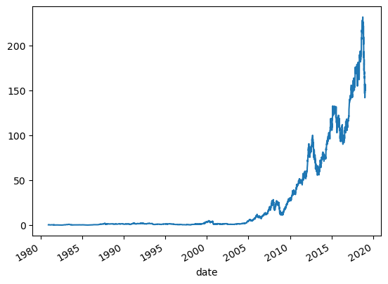
Using dates as index
1
2
3
| sunspots.index = sunspots['year_month_day']
sunspots.index.name = 'date'
sunspots.iloc[10:20, :]
|
| dec_date | tot_sunspots | daily_std | observations | definite | year_month_day |
|---|
| date | | | | | | |
|---|
| 1818-01-11 | 1818.029 | NaN | NaN | 0 | 1 | 1818-01-11 |
|---|
| 1818-01-12 | 1818.032 | NaN | NaN | 0 | 1 | 1818-01-12 |
|---|
| 1818-01-13 | 1818.034 | 37.0 | 7.7 | 1 | 1 | 1818-01-13 |
|---|
| 1818-01-14 | 1818.037 | NaN | NaN | 0 | 1 | 1818-01-14 |
|---|
| 1818-01-15 | 1818.040 | NaN | NaN | 0 | 1 | 1818-01-15 |
|---|
| 1818-01-16 | 1818.042 | NaN | NaN | 0 | 1 | 1818-01-16 |
|---|
| 1818-01-17 | 1818.045 | 77.0 | 11.1 | 1 | 1 | 1818-01-17 |
|---|
| 1818-01-18 | 1818.048 | 98.0 | 12.6 | 1 | 1 | 1818-01-18 |
|---|
| 1818-01-19 | 1818.051 | 105.0 | 13.0 | 1 | 1 | 1818-01-19 |
|---|
| 1818-01-20 | 1818.053 | NaN | NaN | 0 | 1 | 1818-01-20 |
|---|
1
2
3
4
5
6
7
8
9
10
11
12
13
| <class 'pandas.core.frame.DataFrame'>
DatetimeIndex: 73414 entries, 1818-01-01 to 2018-12-31
Data columns (total 6 columns):
# Column Non-Null Count Dtype
--- ------ -------------- -----
0 dec_date 73414 non-null float64
1 tot_sunspots 70167 non-null float64
2 daily_std 70167 non-null float64
3 observations 73414 non-null int64
4 definite 73414 non-null int64
5 year_month_day 73414 non-null datetime64[ns]
dtypes: datetime64[ns](1), float64(3), int64(2)
memory usage: 3.9 MB
|
Trimming redundant columns
1
2
3
| cols = ['tot_sunspots', 'daily_std', 'observations', 'definite']
sunspots = sunspots[cols]
sunspots.iloc[10:20, :]
|
| tot_sunspots | daily_std | observations | definite |
|---|
| date | | | | |
|---|
| 1818-01-11 | NaN | NaN | 0 | 1 |
|---|
| 1818-01-12 | NaN | NaN | 0 | 1 |
|---|
| 1818-01-13 | 37.0 | 7.7 | 1 | 1 |
|---|
| 1818-01-14 | NaN | NaN | 0 | 1 |
|---|
| 1818-01-15 | NaN | NaN | 0 | 1 |
|---|
| 1818-01-16 | NaN | NaN | 0 | 1 |
|---|
| 1818-01-17 | 77.0 | 11.1 | 1 | 1 |
|---|
| 1818-01-18 | 98.0 | 12.6 | 1 | 1 |
|---|
| 1818-01-19 | 105.0 | 13.0 | 1 | 1 |
|---|
| 1818-01-20 | NaN | NaN | 0 | 1 |
|---|
Writing files
1
2
3
4
5
6
| out_csv = 'sunspots.csv'
sunspots.to_csv(out_csv)
out_tsv = 'sunspots.tsv'
sunspots.to_csv(out_tsv, sep='\t')
out_xlsx = 'sunspots.xlsx'
sunspots.to_excel(out_xlsx)
|
Exercises
Reading a flat file
In previous exercises, we have preloaded the data for you using the pandas function read_csv(). Now, it’s your turn! Your job is to read the World Bank population data you saw earlier into a DataFrame using read_csv(). The file is available in the variable data_file.
The next step is to reread the same file, but simultaneously rename the columns using the names keyword input parameter, set equal to a list of new column labels. You will also need to set header=0 to rename the column labels.
Finish up by inspecting the result with df.head() and df.info() in the IPython Shell (changing df to the name of your DataFrame variable).
pandas has already been imported and is available in the workspace as pd.
Instructions
- Use pd.read_csv() with the string data_file to read the CSV file into a DataFrame and assign it to df1.
- Create a list of new column labels - ‘year’, ‘population’ - and assign it to the variable new_labels.
- Reread the same file, again using pd.read_csv(), but this time, add the keyword arguments header=0 and names=new_labels. Assign the resulting DataFrame to df2.
- Print both the df1 and df2 DataFrames to see the change in column names. This has already been done for you.
1
| data_file = 'DataCamp-master/11-pandas-foundations/_datasets/world_population.csv'
|
1
2
| # Read in the file: df1
df1 = pd.read_csv(data_file)
|
1
2
| # Create a list of the new column labels: new_labels
new_labels = ['year', 'population']
|
1
2
| # Read in the file, specifying the header and names parameters: df2
df2 = pd.read_csv(data_file, header=0, names=new_labels)
|
1
2
| # Print both the DataFrames
df1.head()
|
| Date | Total Population |
|---|
| 0 | 1960 | 3034970564 |
|---|
| 1 | 1970 | 3684822701 |
|---|
| 2 | 1980 | 4436590356 |
|---|
| 3 | 1990 | 5282715991 |
|---|
| 4 | 2000 | 6115974486 |
|---|
| year | population |
|---|
| 0 | 1960 | 3034970564 |
|---|
| 1 | 1970 | 3684822701 |
|---|
| 2 | 1980 | 4436590356 |
|---|
| 3 | 1990 | 5282715991 |
|---|
| 4 | 2000 | 6115974486 |
|---|
Delimiters, headers, and extensions
Not all data files are clean and tidy. Pandas provides methods for reading those not-so-perfect data files that you encounter far too often.
In this exercise, you have monthly stock data for four companies downloaded from Yahoo Finance. The data is stored as one row for each company and each column is the end-of-month closing price. The file name is given to you in the variable file_messy.
In addition, this file has three aspects that may cause trouble for lesser tools: multiple header lines, comment records (rows) interleaved throughout the data rows, and space delimiters instead of commas.
Your job is to use pandas to read the data from this problematic file_messy using non-default input options with read_csv() so as to tidy up the mess at read time. Then, write the cleaned up data to a CSV file with the variable file_clean that has been prepared for you, as you might do in a real data workflow.
You can learn about the option input parameters needed by using help() on the pandas function pd.read_csv().
Instructions
- Use pd.read_csv() without using any keyword arguments to read file_messy into a pandas DataFrame df1.
- Use .head() to print the first 5 rows of df1 and see how messy it is. Do this in the IPython Shell first so you can see how modifying read_csv() can clean up this mess.
- Using the keyword arguments delimiter=’ ‘, header=3 and comment=’#’, use pd.read_csv() again to read file_messy into a new DataFrame df2.
- Print the output of df2.head() to verify the file was read correctly.
- Use the DataFrame method .to_csv() to save the DataFrame df2 to the variable file_clean. Be sure to specify index=False.
- Use the DataFrame method .to_excel() to save the DataFrame df2 to the file ‘file_clean.xlsx’. Again, remember to specify index=False
1
2
3
| # Read the raw file as-is: df1
file_messy = 'DataCamp-master/11-pandas-foundations/_datasets/messy_stock_data.tsv'
df1 = pd.read_csv(file_messy)
|
1
2
| # Print the output of df1.head()
df1.head()
|
| The following stock data was collect on 2016-AUG-25 from an unknown source |
|---|
| These kind of ocmments are not very useful | are they? |
|---|
| probably should just throw this line away too | but not the next since those are column labels |
|---|
| name Jan Feb Mar Apr May Jun Jul Aug Sep Oct Nov Dec | NaN |
|---|
| # So that line you just read has all the column headers labels | NaN |
|---|
| IBM 156.08 160.01 159.81 165.22 172.25 167.15 164.75 152.77 145.36 146.11 137.21 137.96 | NaN |
|---|
1
2
| # Read in the file with the correct parameters: df2
df2 = pd.read_csv(file_messy, delimiter=' ', header=3, comment='#')
|
1
2
| # Print the output of df2.head()
df2.head()
|
| name | Jan | Feb | Mar | Apr | May | Jun | Jul | Aug | Sep | Oct | Nov | Dec |
|---|
| 0 | IBM | 156.08 | 160.01 | 159.81 | 165.22 | 172.25 | 167.15 | 164.75 | 152.77 | 145.36 | 146.11 | 137.21 | 137.96 |
|---|
| 1 | MSFT | 45.51 | 43.08 | 42.13 | 43.47 | 47.53 | 45.96 | 45.61 | 45.51 | 43.56 | 48.70 | 53.88 | 55.40 |
|---|
| 2 | GOOGLE | 512.42 | 537.99 | 559.72 | 540.50 | 535.24 | 532.92 | 590.09 | 636.84 | 617.93 | 663.59 | 735.39 | 755.35 |
|---|
| 3 | APPLE | 110.64 | 125.43 | 125.97 | 127.29 | 128.76 | 127.81 | 125.34 | 113.39 | 112.80 | 113.36 | 118.16 | 111.73 |
|---|
save files
1
2
3
4
| # Save the cleaned up DataFrame to a CSV file without the index
df2.to_csv(file_clean, index=False)
# Save the cleaned up DataFrame to an excel file without the index
df2.to_excel('file_clean.xlsx', index=False)
|
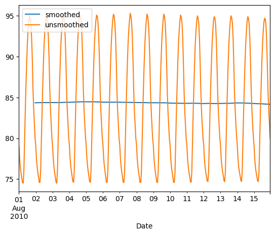
Plotting with Pandas
1
2
3
4
5
6
7
| cols = ['date', 'open', 'high', 'low', 'close', 'adj_close', 'volume']
aapl = pd.read_csv(r'DataCamp-master/11-pandas-foundations/_datasets/AAPL.csv',
names=cols,
index_col='date',
parse_dates=True,
header=0,
na_values='null')
|
| open | high | low | close | adj_close | volume |
|---|
| date | | | | | | |
|---|
| 1980-12-12 | 0.513393 | 0.515625 | 0.513393 | 0.513393 | 0.023106 | 117258400.0 |
|---|
| 1980-12-15 | 0.488839 | 0.488839 | 0.486607 | 0.486607 | 0.021900 | 43971200.0 |
|---|
| 1980-12-16 | 0.453125 | 0.453125 | 0.450893 | 0.450893 | 0.020293 | 26432000.0 |
|---|
| 1980-12-17 | 0.462054 | 0.464286 | 0.462054 | 0.462054 | 0.020795 | 21610400.0 |
|---|
| 1980-12-18 | 0.475446 | 0.477679 | 0.475446 | 0.475446 | 0.021398 | 18362400.0 |
|---|
1
2
3
4
5
6
7
8
9
10
11
12
13
| <class 'pandas.core.frame.DataFrame'>
DatetimeIndex: 9611 entries, 1980-12-12 to 2019-01-24
Data columns (total 6 columns):
# Column Non-Null Count Dtype
--- ------ -------------- -----
0 open 9610 non-null float64
1 high 9610 non-null float64
2 low 9610 non-null float64
3 close 9610 non-null float64
4 adj_close 9610 non-null float64
5 volume 9610 non-null float64
dtypes: float64(6)
memory usage: 525.6 KB
|
| open | high | low | close | adj_close | volume |
|---|
| date | | | | | | |
|---|
| 2019-01-17 | 154.199997 | 157.660004 | 153.259995 | 155.860001 | 155.860001 | 29821200.0 |
|---|
| 2019-01-18 | 157.500000 | 157.880005 | 155.979996 | 156.820007 | 156.820007 | 33751000.0 |
|---|
| 2019-01-22 | 156.410004 | 156.729996 | 152.619995 | 153.300003 | 153.300003 | 30394000.0 |
|---|
| 2019-01-23 | 154.149994 | 155.139999 | 151.699997 | 153.919998 | 153.919998 | 23130600.0 |
|---|
| 2019-01-24 | 154.110001 | 154.479996 | 151.740005 | 152.699997 | 152.699997 | 25421800.0 |
|---|
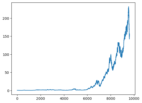
Plotting arrays (matplotlib)
1
| close_arr = aapl['close'].values
|
1
| [<matplotlib.lines.Line2D at 0x19978c3eed0>]
|
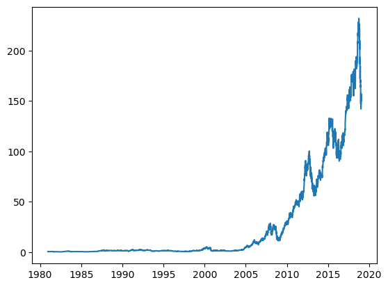
Plotting Series (matplotlib)
1
| close_series = aapl['close']
|
1
| pandas.core.series.Series
|
1
| [<matplotlib.lines.Line2D at 0x199798f5f40>]
|
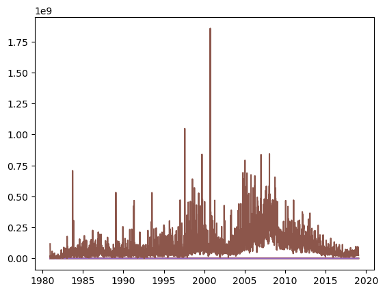
Plotting Series (pandas)
Plotting DataFrames (pandas)
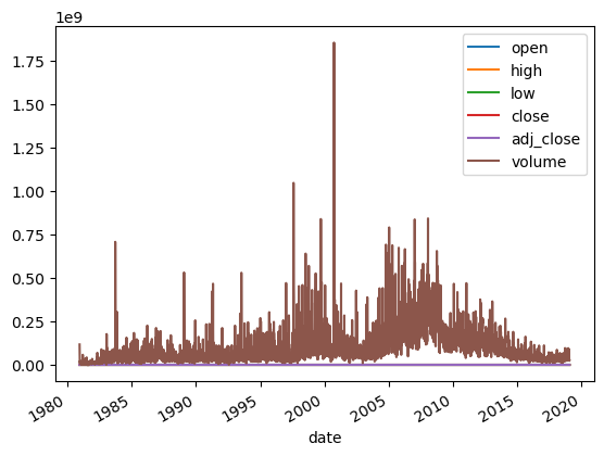
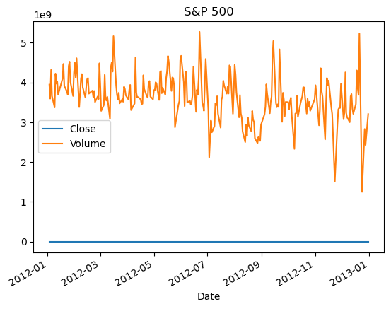
Plotting DataFrames (matplotlib)
1
2
3
4
5
6
| [<matplotlib.lines.Line2D at 0x19978d07350>,
<matplotlib.lines.Line2D at 0x19978bf7dd0>,
<matplotlib.lines.Line2D at 0x19978c8d760>,
<matplotlib.lines.Line2D at 0x199791eea20>,
<matplotlib.lines.Line2D at 0x199791ee900>,
<matplotlib.lines.Line2D at 0x19978c85910>]
|
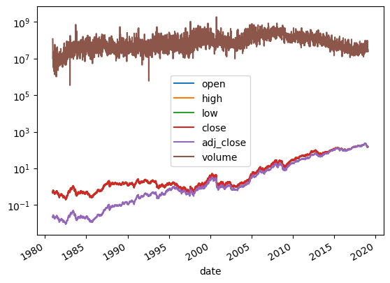
Fixing Scales
1
2
3
| aapl.plot()
plt.yscale('log')
plt.show()
|
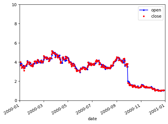
Customizing plots
1
2
3
4
| aapl['open'].plot(color='b', style='.-', legend=True)
aapl['close'].plot(color='r', style='.', legend=True)
plt.axis(('2000', '2001', 0, 10))
plt.show()
|
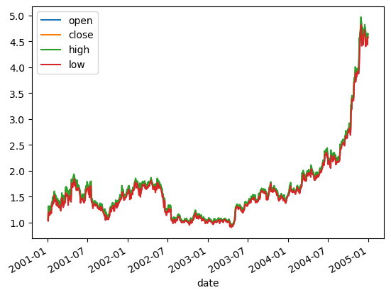
Saving Plots
1
2
3
4
5
6
7
| aapl.loc['2001':'2004', ['open', 'close', 'high', 'low']].plot()
plt.savefig('aapl.png')
plt.savefig('aapl.jpg')
plt.savefig('aapl.pdf')
plt.show()
|
Exercises
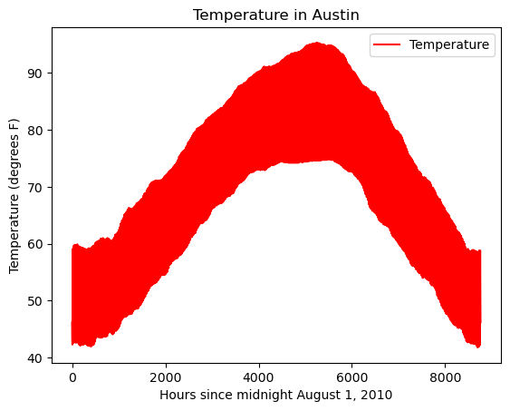
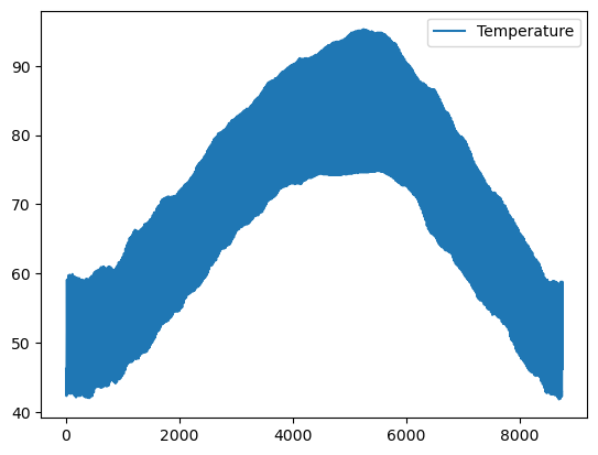
Plotting series using pandas
Data visualization is often a very effective first step in gaining a rough understanding of a data set to be analyzed. Pandas provides data visualization by both depending upon and interoperating with the matplotlib library. You will now explore some of the basic plotting mechanics with pandas as well as related matplotlib options. We have pre-loaded a pandas DataFrame df which contains the data you need. Your job is to use the DataFrame method df.plot() to visualize the data, and then explore the optional matplotlib input parameters that this .plot() method accepts.
The pandas .plot() method makes calls to matplotlib to construct the plots. This means that you can use the skills you’ve learned in previous visualization courses to customize the plot. In this exercise, you’ll add a custom title and axis labels to the figure.
Before plotting, inspect the DataFrame in the IPython Shell using df.head(). Also, use type(df) and note that it is a single column DataFrame.
Instructions
- Create the plot with the DataFrame method df.plot(). Specify a color of ‘red’.
- Note: c and color are interchangeable as parameters here, but we ask you to be explicit and specify color.
- Use plt.title() to give the plot a title of ‘Temperature in Austin’.
- Use plt.xlabel() to give the plot an x-axis label of ‘Hours since midnight August 1, 2010’.
- Use plt.ylabel() to give the plot a y-axis label of ‘Temperature (degrees F)’.
- Finally, display the plot using plt.show()
1
2
| data_file = 'DataCamp-master/11-pandas-foundations/_datasets/weather_data_austin_2010.csv'
df = pd.read_csv(data_file, usecols=['Temperature'])
|
1
2
3
4
5
6
7
8
| <class 'pandas.core.frame.DataFrame'>
RangeIndex: 8759 entries, 0 to 8758
Data columns (total 1 columns):
# Column Non-Null Count Dtype
--- ------ -------------- -----
0 Temperature 8759 non-null float64
dtypes: float64(1)
memory usage: 68.6 KB
|
| Temperature |
|---|
| 0 | 46.2 |
|---|
| 1 | 44.6 |
|---|
| 2 | 44.1 |
|---|
| 3 | 43.8 |
|---|
| 4 | 43.5 |
|---|
1
2
3
4
5
6
7
8
9
10
11
12
13
14
| # Create a plot with color='red'
df.plot(color='r')
# Add a title
plt.title('Temperature in Austin')
# Specify the x-axis label
plt.xlabel('Hours since midnight August 1, 2010')
# Specify the y-axis label
plt.ylabel('Temperature (degrees F)')
# Display the plot
plt.show()
|
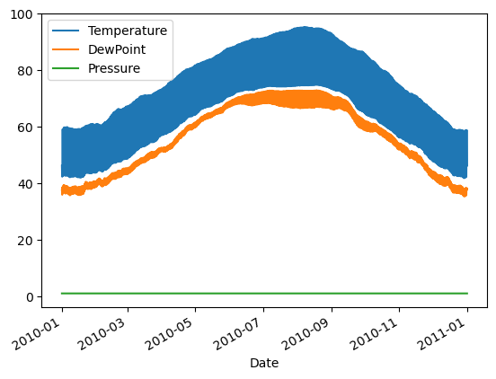
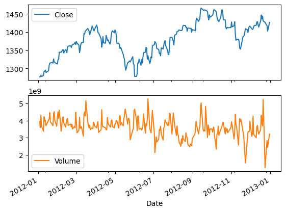
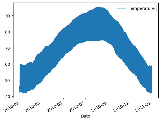
Plotting DataFrames
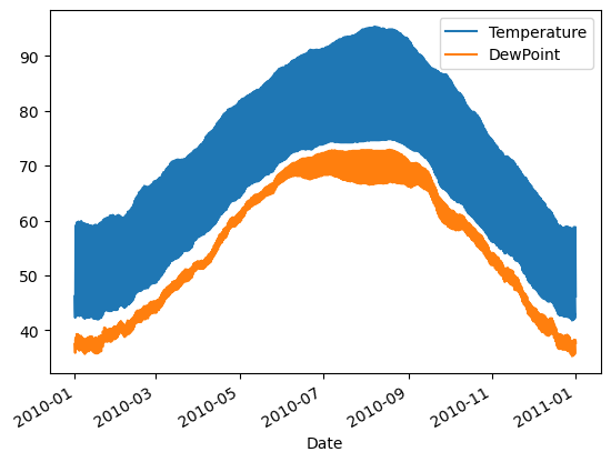
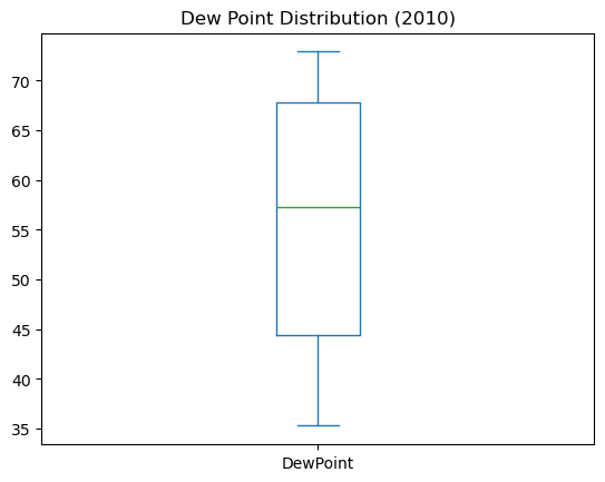
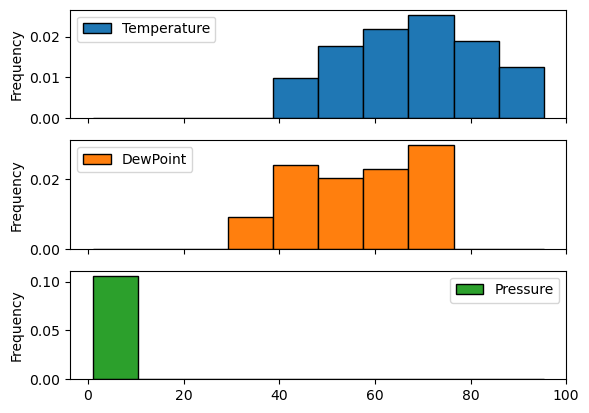
Comparing data from several columns can be very illuminating. Pandas makes doing so easy with multi-column DataFrames. By default, calling df.plot() will cause pandas to over-plot all column data, with each column as a single line. In this exercise, we have pre-loaded three columns of data from a weather data set - temperature, dew point, and pressure - but the problem is that pressure has different units of measure. The pressure data, measured in Atmospheres, has a different vertical scaling than that of the other two data columns, which are both measured in degrees Fahrenheit.
Your job is to plot all columns as a multi-line plot, to see the nature of vertical scaling problem. Then, use a list of column names passed into the DataFrame df[column_list] to limit plotting to just one column, and then just 2 columns of data. When you are finished, you will have created 4 plots. You can cycle through them by clicking on the ‘Previous Plot’ and ‘Next Plot’ buttons.
As in the previous exercise, inspect the DataFrame df in the IPython Shell using the .head() and .info() methods.
Instructions
- Plot all columns together on one figure by calling df.plot(), and noting the vertical scaling problem.
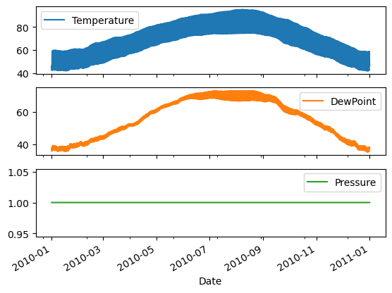
- Plot all columns as subplots. To do so, you need to specify subplots=True inside .plot().
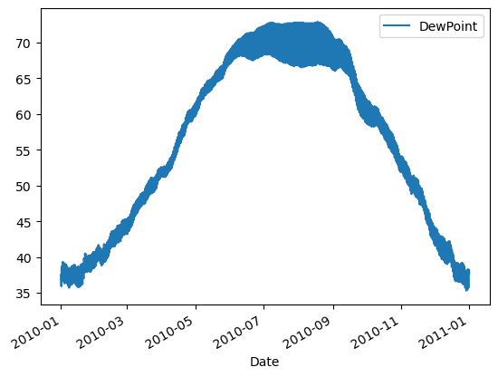
- Plot a single column of dew point data. To do this, define a column list containing a single column name ‘Dew Point (deg F)’, and call df[column_list1].plot().
- Plot two columns of data, ‘Temperature (deg F)’ and ‘Dew Point (deg F)’. To do this, define a list containing those column names and pass it into df[], as df[column_list2].plot().
1
2
3
| data_file = 'DataCamp-master/11-pandas-foundations/_datasets/weather_data_austin_2010.csv'
df = pd.read_csv(data_file, parse_dates=[3], index_col='Date')
df.head()
|
| Temperature | DewPoint | Pressure |
|---|
| Date | | | |
|---|
| 2010-01-01 00:00:00 | 46.2 | 37.5 | 1.0 |
|---|
| 2010-01-01 01:00:00 | 44.6 | 37.1 | 1.0 |
|---|
| 2010-01-01 02:00:00 | 44.1 | 36.9 | 1.0 |
|---|
| 2010-01-01 03:00:00 | 43.8 | 36.9 | 1.0 |
|---|
| 2010-01-01 04:00:00 | 43.5 | 36.8 | 1.0 |
|---|
1
2
3
| # Plot all columns (default)
df.plot()
plt.show()
|
1
2
3
| # Plot all columns as subplots
df.plot(subplots=True)
plt.show()
|
1
2
3
4
| # Plot just the Dew Point data
column_list1 = ['DewPoint']
df[column_list1].plot()
plt.show()
|
1
2
3
4
| # Plot the Dew Point and Temperature data, but not the Pressure data
column_list2 = ['Temperature','DewPoint']
df[column_list2].plot()
plt.show()
|
Exploratory Data Analysis
Having learned how to ingest and inspect your data, you will next explore it visually as well as quantitatively. This process, known as exploratory data analysis (EDA), is a crucial component of any data science project. Pandas has powerful methods that help with statistical and visual EDA. In this chapter, you will learn how and when to apply these techniques.
Visual exploratory data analysis
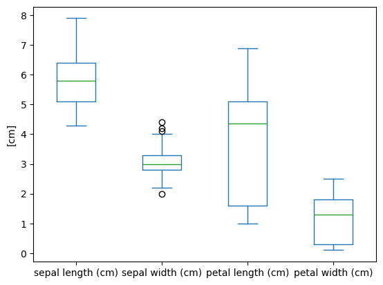
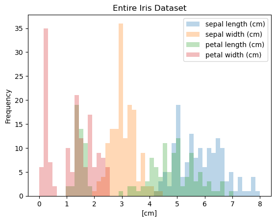
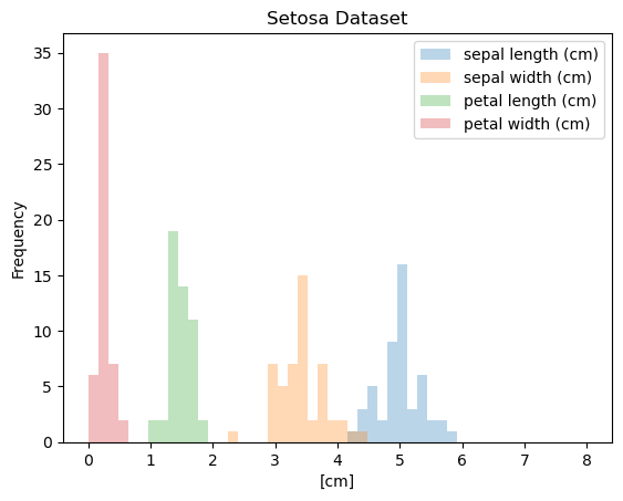
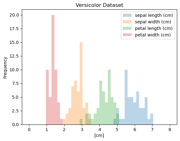
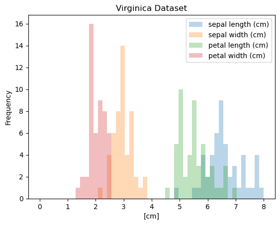
The Iris Dataset
- Famous dataset in pattern recognition
- 150 observations, 4 features each
- Sepal length
- Sepal width
- Petal length
- Petal width
- 3 species:
- setosa
- versicolor
- virginica
1
2
| data_file = 'DataCamp-master/11-pandas-foundations/_datasets/iris.csv'
iris = pd.read_csv(data_file)
|
| sepal length (cm) | sepal width (cm) | petal length (cm) | petal width (cm) | species |
|---|
| 0 | 5.1 | 3.5 | 1.4 | 0.2 | setosa |
|---|
| 1 | 4.9 | 3.0 | 1.4 | 0.2 | setosa |
|---|
| 2 | 4.7 | 3.2 | 1.3 | 0.2 | setosa |
|---|
| 3 | 4.6 | 3.1 | 1.5 | 0.2 | setosa |
|---|
| 4 | 5.0 | 3.6 | 1.4 | 0.2 | setosa |
|---|
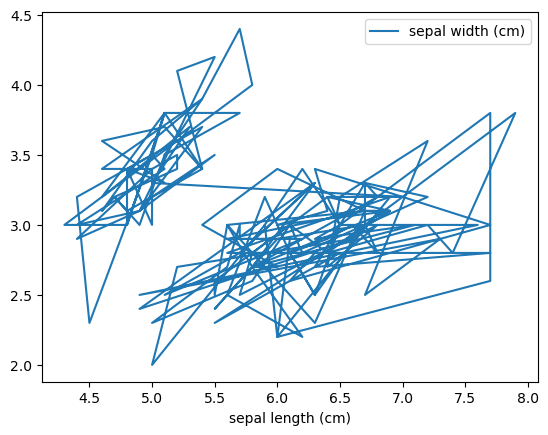
Line plot
1
| iris.plot(x='sepal length (cm)', y='sepal width (cm)')
|
1
| <Axes: xlabel='sepal length (cm)'>
|
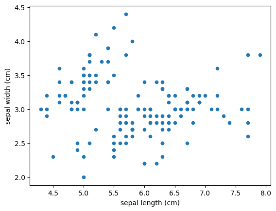
Scatter Plot
1
2
3
4
| iris.plot(x='sepal length (cm)', y='sepal width (cm)',
kind='scatter')
plt.xlabel('sepal length (cm)')
plt.ylabel('sepal width (cm)')
|
1
| Text(0, 0.5, 'sepal width (cm)')
|
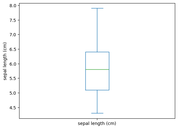
Box Plot
1
2
3
| iris.plot(y='sepal length (cm)',
kind='box')
plt.ylabel('sepal length (cm)')
|
1
| Text(0, 0.5, 'sepal length (cm)')
|
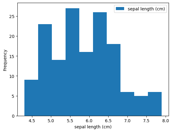
Histogram
1
2
3
| iris.plot(y='sepal length (cm)',
kind='hist')
plt.xlabel('sepal length (cm)')
|
1
| Text(0.5, 0, 'sepal length (cm)')
|
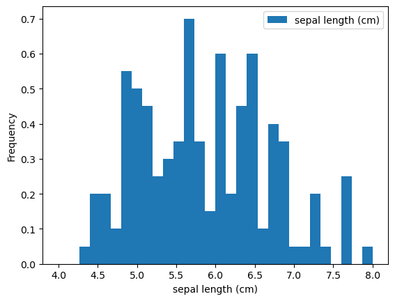
Histogram Options
- bins (integer): number of intervals or bins
- range (tuple): extrema of bins (minimum, maximum)
- density (boolean): whether to normalized to one - formerly this was normed
- cumulative (boolean): computer Cumulative Distributions Function (CDF)
- … more matplotlib customizations
Customizing Histogram
1
2
3
4
5
6
| iris.plot(y='sepal length (cm)',
kind='hist',
bins=30,
range=(4, 8),
density=True)
plt.xlabel('sepal length (cm)')
|
1
| Text(0.5, 0, 'sepal length (cm)')
|
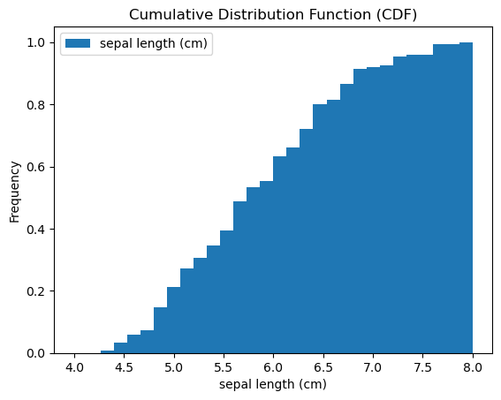
Cumulative Distribution
1
2
3
4
5
6
7
8
| iris.plot(y='sepal length (cm)',
kind='hist',
bins=30,
range=(4, 8),
density=True,
cumulative=True)
plt.xlabel('sepal length (cm)')
plt.title('Cumulative Distribution Function (CDF)')
|
1
| Text(0.5, 1.0, 'Cumulative Distribution Function (CDF)')
|
Word of Warning
- Three different DataFrame plot idioms
- iris.plot(kind=’hist’)
- iris.plt.hist()
- iris.hist()
- Syntax / Results differ!
- Pandas API still evolving: chech the documentation
Exercises
pandas line plots
In the previous chapter, you saw that the .plot() method will place the Index values on the x-axis by default. In this exercise, you’ll practice making line plots with specific columns on the x and y axes.
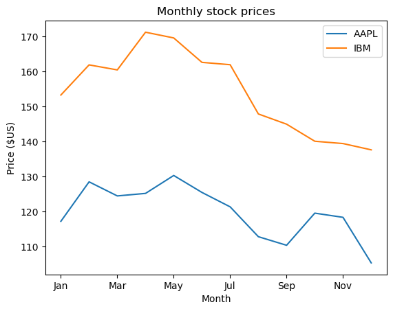
You will work with a dataset consisting of monthly stock prices in 2015 for AAPL, GOOG, and IBM. The stock prices were obtained from Yahoo Finance. Your job is to plot the ‘Month’ column on the x-axis and the AAPL and IBM prices on the y-axis using a list of column names.
All necessary modules have been imported for you, and the DataFrame is available in the workspace as df. Explore it using methods such as .head(), .info(), and .describe() to see the column names.
Instructions
- Create a list of y-axis column names called y_columns consisting of ‘AAPL’ and ‘IBM’.
- Generate a line plot with x=’Month’ and y=y_columns as inputs.
- Give the plot a title of ‘Monthly stock prices’.
- Specify the y-axis label.
- Display the plot.
1
2
3
4
5
6
7
8
9
10
11
12
13
14
| values = [['Jan', 117.160004, 534.5224450000002, 153.309998],
['Feb', 128.46000700000002, 558.402511, 161.940002],
['Mar', 124.43, 548.002468, 160.5],
['Apr', 125.150002, 537.340027, 171.28999299999995],
['May', 130.279999, 532.1099849999998, 169.649994],
['Jun', 125.43, 520.51001, 162.660004],
['Jul', 121.300003, 625.6099849999998, 161.990005],
['Aug', 112.760002, 618.25, 147.889999],
['Sep', 110.300003, 608.419983, 144.970001],
['Oct', 119.5, 710.8099980000002, 140.080002],
['Nov', 118.300003, 742.599976, 139.419998],
['Dec', 105.260002, 758.880005, 137.619995]]
values = np.array(values).transpose()
|
1
| cols = ['Month', 'AAPL', 'GOOG', 'IBM']
|
1
| data_zipped = list(zip(cols, values))
|
1
| data_dict = dict(data_zipped)
|
1
| dtype = dict(zip(data_dict.keys(), ['str', 'float64', 'float64', 'float64']))
|
1
| {'Month': 'str', 'AAPL': 'float64', 'GOOG': 'float64', 'IBM': 'float64'}
|
1
| df = pd.DataFrame.from_dict(data_dict).astype(dtype)
|
| Month | AAPL | GOOG | IBM |
|---|
| 0 | Jan | 117.160004 | 534.522445 | 153.309998 |
|---|
| 1 | Feb | 128.460007 | 558.402511 | 161.940002 |
|---|
| 2 | Mar | 124.430000 | 548.002468 | 160.500000 |
|---|
| 3 | Apr | 125.150002 | 537.340027 | 171.289993 |
|---|
| 4 | May | 130.279999 | 532.109985 | 169.649994 |
|---|
| 5 | Jun | 125.430000 | 520.510010 | 162.660004 |
|---|
| 6 | Jul | 121.300003 | 625.609985 | 161.990005 |
|---|
| 7 | Aug | 112.760002 | 618.250000 | 147.889999 |
|---|
| 8 | Sep | 110.300003 | 608.419983 | 144.970001 |
|---|
| 9 | Oct | 119.500000 | 710.809998 | 140.080002 |
|---|
| 10 | Nov | 118.300003 | 742.599976 | 139.419998 |
|---|
| 11 | Dec | 105.260002 | 758.880005 | 137.619995 |
|---|
1
2
3
4
5
6
7
8
9
10
11
| <class 'pandas.core.frame.DataFrame'>
RangeIndex: 12 entries, 0 to 11
Data columns (total 4 columns):
# Column Non-Null Count Dtype
--- ------ -------------- -----
0 Month 12 non-null object
1 AAPL 12 non-null float64
2 GOOG 12 non-null float64
3 IBM 12 non-null float64
dtypes: float64(3), object(1)
memory usage: 516.0+ bytes
|
1
2
3
4
5
6
7
8
9
10
11
12
13
14
| # Create a list of y-axis column names: y_columns
y_columns = ['AAPL', 'IBM']
# Generate a line plot
df.plot(x='Month', y=y_columns)
# Add the title
plt.title('Monthly stock prices')
# Add the y-axis label
plt.ylabel('Price ($US)')
# Display the plot
plt.show()
|
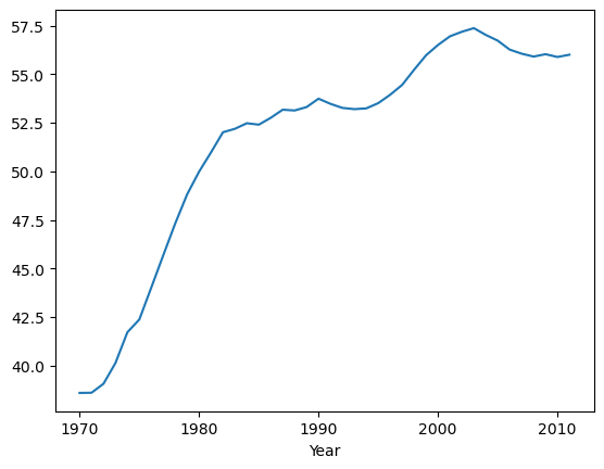
pandas scatter plots
Pandas scatter plots are generated using the kind='scatter' keyword argument. Scatter plots require that the x and y columns be chosen by specifying the x and y parameters inside .plot(). Scatter plots also take an s keyword argument to provide the radius of each circle to plot in pixels.
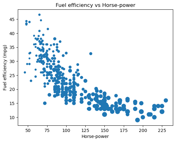
In this exercise, you’re going to plot fuel efficiency (miles-per-gallon) versus horse-power for 392 automobiles manufactured from 1970 to 1982 from the UCI Machine Learning Repository.
The size of each circle is provided as a NumPy array called sizes. This array contains the normalized 'weight' of each automobile in the dataset.
All necessary modules have been imported and the DataFrame is available in the workspace as df.
Instructions
- Generate a scatter plot with ‘hp’ on the x-axis and ‘mpg’ on the y-axis. Specify s=sizes.
- Add a title to the plot.
- Specify the x-axis and y-axis labels.
1
2
3
| data_file = 'DataCamp-master/11-pandas-foundations/_datasets/auto-mpg.csv'
df = pd.read_csv(data_file)
df.head()
|
| mpg | cyl | displ | hp | weight | accel | yr | origin | name |
|---|
| 0 | 18.0 | 8 | 307.0 | 130 | 3504 | 12.0 | 70 | US | chevrolet chevelle malibu |
|---|
| 1 | 15.0 | 8 | 350.0 | 165 | 3693 | 11.5 | 70 | US | buick skylark 320 |
|---|
| 2 | 18.0 | 8 | 318.0 | 150 | 3436 | 11.0 | 70 | US | plymouth satellite |
|---|
| 3 | 16.0 | 8 | 304.0 | 150 | 3433 | 12.0 | 70 | US | amc rebel sst |
|---|
| 4 | 17.0 | 8 | 302.0 | 140 | 3449 | 10.5 | 70 | US | ford torino |
|---|
1
2
3
4
5
6
7
8
9
10
11
12
13
14
15
16
| <class 'pandas.core.frame.DataFrame'>
RangeIndex: 392 entries, 0 to 391
Data columns (total 9 columns):
# Column Non-Null Count Dtype
--- ------ -------------- -----
0 mpg 392 non-null float64
1 cyl 392 non-null int64
2 displ 392 non-null float64
3 hp 392 non-null int64
4 weight 392 non-null int64
5 accel 392 non-null float64
6 yr 392 non-null int64
7 origin 392 non-null object
8 name 392 non-null object
dtypes: float64(3), int64(4), object(2)
memory usage: 27.7+ KB
|
1
2
3
4
5
6
7
8
9
10
11
12
13
14
15
16
17
18
19
20
21
22
23
24
25
26
27
28
29
30
31
32
33
34
35
36
37
38
39
40
41
42
43
44
45
46
47
48
49
50
51
52
53
54
55
56
57
58
59
60
61
62
63
64
65
66
67
68
69
70
71
72
73
74
75
76
77
78
79
80
81
82
83
84
85
86
87
88
89
90
91
92
93
94
95
96
97
98
| sizes = np.array([ 51.12044694, 56.78387977, 49.15557238, 49.06977358,
49.52823321, 78.4595872 , 78.93021696, 77.41479205,
81.52541106, 61.71459825, 52.85646225, 54.23007578,
58.89427963, 39.65137852, 23.42587473, 33.41639502,
32.03903011, 27.8650165 , 18.88972581, 14.0196956 ,
29.72619722, 24.58549713, 23.48516821, 20.77938954,
29.19459189, 88.67676838, 79.72987328, 79.94866084,
93.23005042, 18.88972581, 21.34122243, 20.6679223 ,
28.88670381, 49.24144612, 46.14174741, 45.39631334,
45.01218186, 73.76057586, 82.96880195, 71.84547684,
69.85320595, 102.22421043, 93.78252358, 110. ,
36.52889673, 24.14234281, 44.84805372, 41.02504618,
20.51976563, 18.765772 , 17.9095202 , 17.75442285,
13.08832041, 10.83266174, 14.00441945, 15.91328975,
21.60597587, 18.8188451 , 21.15311208, 24.14234281,
20.63083317, 76.05635059, 80.05816704, 71.18975117,
70.98330444, 56.13992036, 89.36985382, 84.38736544,
82.6716892 , 81.4149056 , 22.60363518, 63.06844313,
69.92143863, 76.76982089, 69.2066568 , 35.81711267,
26.25184749, 36.94940537, 19.95069229, 23.88237331,
21.79608472, 26.1474042 , 19.49759118, 18.36136808,
69.98970461, 56.13992036, 66.21810474, 68.02351436,
59.39644014, 102.10046481, 82.96880195, 79.25686195,
74.74521151, 93.34830013, 102.05923292, 60.7883734 ,
40.55589449, 44.7388015 , 36.11079464, 37.9986264 ,
35.11233175, 15.83199594, 103.96451839, 100.21241654,
90.18186347, 84.27493641, 32.38645967, 21.62494928,
24.00218436, 23.56434276, 18.78345471, 22.21725537,
25.44271071, 21.36007926, 69.37650986, 76.19877818,
14.51292942, 19.38962134, 27.75740889, 34.24717407,
48.10262495, 29.459795 , 32.80584831, 55.89556844,
40.06360581, 35.03982309, 46.33599903, 15.83199594,
25.01226779, 14.03498009, 26.90404245, 59.52231336,
54.92349014, 54.35035315, 71.39649768, 91.93424995,
82.70879915, 89.56285636, 75.45251972, 20.50128352,
16.04379287, 22.02531454, 11.32159874, 16.70430249,
18.80114574, 18.50153068, 21.00322336, 25.79385418,
23.80266582, 16.65430211, 44.35746794, 49.815853 ,
49.04119063, 41.52318884, 90.72524338, 82.07906251,
84.23747672, 90.29816462, 63.55551901, 63.23059357,
57.92740995, 59.64831981, 38.45278922, 43.19643409,
41.81296121, 19.62393488, 28.99647648, 35.35456858,
27.97283229, 30.39744886, 20.57526193, 26.96758278,
37.07354237, 15.62160631, 42.92863291, 30.21771564,
36.40567571, 36.11079464, 29.70395123, 13.41514444,
25.27829944, 20.51976563, 27.54281821, 21.17188565,
20.18836167, 73.97101962, 73.09614831, 65.35749368,
73.97101962, 43.51889468, 46.80945169, 37.77255674,
39.6256851 , 17.24230306, 19.49759118, 15.62160631,
13.41514444, 55.49963323, 53.18333207, 55.31736854,
42.44868923, 13.86730874, 16.48817545, 19.33574884,
27.3931002 , 41.31307817, 64.63368105, 44.52069676,
35.74387954, 60.75655952, 79.87569835, 68.46177648,
62.35745431, 58.70651902, 17.41217694, 19.33574884,
13.86730874, 22.02531454, 15.75091031, 62.68013142,
68.63071356, 71.36201911, 76.80558184, 51.58836621,
48.84134317, 54.86301837, 51.73502816, 74.14661842,
72.22648148, 77.88228247, 78.24284811, 15.67003285,
31.25845963, 21.36007926, 31.60164234, 17.51450098,
17.92679488, 16.40542438, 19.96892459, 32.99310928,
28.14577056, 30.80379718, 16.40542438, 13.48998471,
16.40542438, 17.84050478, 13.48998471, 47.1451025 ,
58.08281541, 53.06435374, 52.02897659, 41.44433489,
36.60292926, 30.80379718, 48.98404972, 42.90189859,
47.56635225, 39.24128299, 54.56115914, 48.41447259,
48.84134317, 49.41341845, 42.76835191, 69.30854366,
19.33574884, 27.28640858, 22.02531454, 20.70504474,
26.33555201, 31.37264569, 33.93740821, 24.08222494,
33.34566004, 41.05118927, 32.52595611, 48.41447259,
16.48817545, 18.97851406, 43.84255439, 37.22278157,
34.77459916, 44.38465193, 47.00510227, 61.39441929,
57.77221268, 65.12675249, 61.07507305, 79.14790534,
68.42801405, 54.10993164, 64.63368105, 15.42864956,
16.24054679, 15.26876826, 29.68171358, 51.88189829,
63.32798377, 42.36896092, 48.6988448 , 20.15170555,
19.24612787, 16.98905358, 18.88972581, 29.68171358,
28.03762169, 30.35246559, 27.20120517, 19.13885751,
16.12562794, 18.71277385, 16.9722369 , 29.85984799,
34.29495526, 37.54716158, 47.59450219, 19.93246832,
30.60028577, 26.90404245, 24.66650366, 21.36007926,
18.5366546 , 32.64243213, 18.5366546 , 18.09999962,
22.70075058, 36.23351603, 43.97776651, 14.24983724,
19.15671509, 14.17291518, 35.25757392, 24.38356372,
26.02234705, 21.83420642, 25.81458463, 28.90864169,
28.58044785, 30.91715052, 23.6833544 , 12.82391671,
14.63757021, 12.89709155, 17.75442285, 16.24054679,
17.49742615, 16.40542438, 20.42743834, 17.41217694,
23.58415722, 19.96892459, 20.33531923, 22.99334585,
28.47146626, 28.90864169, 43.43816712, 41.57579979,
35.01567018, 35.74387954, 48.5565546 , 57.77221268,
38.98605581, 49.98882458, 28.25412762, 29.01845599,
23.88237331, 27.60710798, 26.54539622, 31.14448175,
34.17556473, 16.3228815 , 17.0732619 , 16.15842026,
18.80114574, 18.80114574, 19.42557798, 20.2434083 ,
20.98452475, 16.07650192, 16.07650192, 16.57113469,
36.11079464, 37.84783835, 27.82194848, 33.46359332,
29.5706502 , 23.38638738, 36.23351603, 32.40968826,
18.88972581, 21.92965639, 28.68963762, 30.80379718])
|
1
2
3
4
5
6
7
8
9
10
11
12
13
14
| # Generate a scatter plot
df.plot(kind='scatter', x='hp', y='mpg', s=sizes)
# Add the title
plt.title('Fuel efficiency vs Horse-power')
# Add the x-axis label
plt.xlabel('Horse-power')
# Add the y-axis label
plt.ylabel('Fuel efficiency (mpg)')
# Display the plot
plt.show()
|
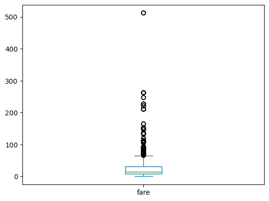
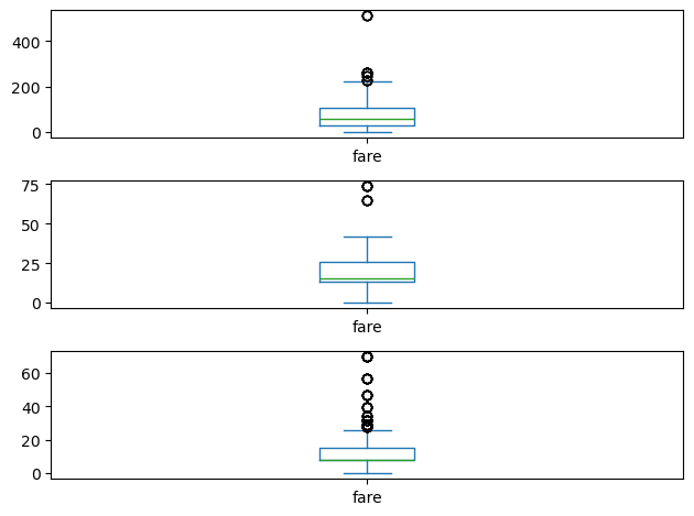
pandas box plots
While pandas can plot multiple columns of data in a single figure, making plots that share the same x and y axes, there are cases where two columns cannot be plotted together because their units do not match. The .plot() method can generate subplots for each column being plotted. Here, each plot will be scaled independently.
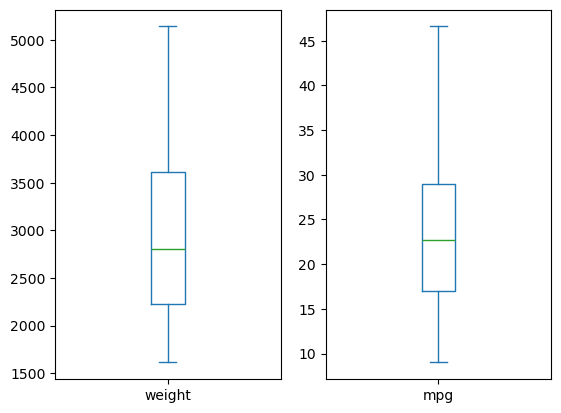
In this exercise your job is to generate box plots for fuel efficiency (mpg) and weight from the automobiles data set. To do this in a single figure, you’ll specify subplots=True inside .plot() to generate two separate plots.
All necessary modules have been imported and the automobiles dataset is available in the workspace as df.
Instructions
- Make a list called cols of the column names to be plotted: ‘weight’ and ‘mpg’.
- Call plot on df[cols] to generate a box plot of the two columns in a single figure. To do this, specify subplots=True.
1
2
3
4
5
6
7
8
| # Make a list of the column names to be plotted: cols
cols = ['weight', 'mpg']
# Generate the box plots
df[cols].plot(kind='box', subplots=True)
# Display the plot
plt.show()
|
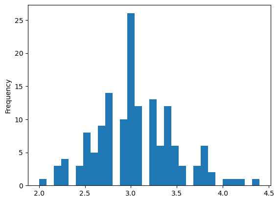
pandas hist, pdf and cd
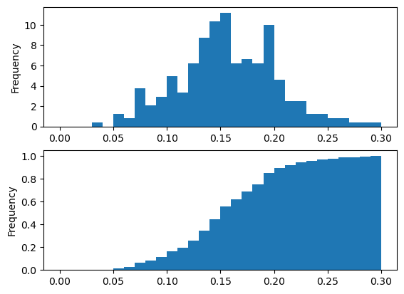
Pandas relies on the .hist() method to not only generate histograms, but also plots of probability density functions (PDFs) and cumulative density functions (CDFs).
In this exercise, you will work with a dataset consisting of restaurant bills that includes the amount customers tipped.
The original dataset is provided by the Seaborn package.
Your job is to plot a PDF and CDF for the fraction column of the tips dataset. This column contains information about what fraction of the total bill is comprised of the tip.
Remember, when plotting the PDF, you need to specify normed=True in your call to .hist(), and when plotting the CDF, you need to specify cumulative=True in addition to normed=True.
All necessary modules have been imported and the tips dataset is available in the workspace as df. Also, some formatting code has been written so that the plots you generate will appear on separate rows.
Instructions
- Plot a PDF for the values in fraction with 30 bins between 0 and 30%. The range has been taken care of for you. ax=axes[0] means that this plot will appear in the first row.
- Plot a CDF for the values in fraction with 30 bins between 0 and 30%. Again, the range has been specified for you. To make the CDF appear on the second row, you need to specify ax=axes[1].
1
2
3
| data_file = 'DataCamp-master/11-pandas-foundations/_datasets/tips.csv'
df = pd.read_csv(data_file)
df.head()
|
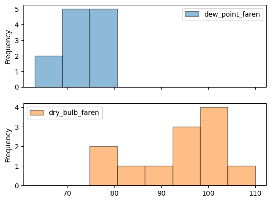
| total_bill | tip | sex | smoker | day | time | size | fraction |
|---|
| 0 | 16.99 | 1.01 | Female | No | Sun | Dinner | 2 | 0.059447 |
|---|
| 1 | 10.34 | 1.66 | Male | No | Sun | Dinner | 3 | 0.160542 |
|---|
| 2 | 21.01 | 3.50 | Male | No | Sun | Dinner | 3 | 0.166587 |
|---|
| 3 | 23.68 | 3.31 | Male | No | Sun | Dinner | 2 | 0.139780 |
|---|
| 4 | 24.59 | 3.61 | Female | No | Sun | Dinner | 4 | 0.146808 |
|---|
1
2
3
4
5
6
7
8
| # This formats the plots such that they appear on separate rows
fig, axes = plt.subplots(nrows=2, ncols=1)
# Plot the PDF
df.fraction.plot(ax=axes[0], kind='hist', bins=30, density=True, range=(0,.3))
# Plot the CDF
df.fraction.plot(ax=axes[1], kind='hist', bins=30, density=True, cumulative=True, range=(0,.3))
|
1
| <Axes: ylabel='Frequency'>
|
Statistical Exploratory Data Analysis
Summarizing with describe()
Describe
- count: number of entires
- mean: average of entries
- std: standard deviation
- min: miniumum entry
- 25%: first quartile
- 50%: median or second quartile
- 75%: third quartile
- max: maximum entry
1
| iris.describe() # summary statistics
|
| sepal length (cm) | sepal width (cm) | petal length (cm) | petal width (cm) |
|---|
| count | 150.000000 | 150.000000 | 150.000000 | 150.000000 |
|---|
| mean | 5.843333 | 3.054000 | 3.758667 | 1.198667 |
|---|
| std | 0.828066 | 0.433594 | 1.764420 | 0.763161 |
|---|
| min | 4.300000 | 2.000000 | 1.000000 | 0.100000 |
|---|
| 25% | 5.100000 | 2.800000 | 1.600000 | 0.300000 |
|---|
| 50% | 5.800000 | 3.000000 | 4.350000 | 1.300000 |
|---|
| 75% | 6.400000 | 3.300000 | 5.100000 | 1.800000 |
|---|
| max | 7.900000 | 4.400000 | 6.900000 | 2.500000 |
|---|
Counts
1
| iris['sepal length (cm)'].count() # Applied to Series
|
1
| iris['sepal width (cm)'].count() # Applied to Series
|
1
| iris[['petal length (cm)', 'petal width (cm)']].count() # Applied to DataFrame
|
1
2
3
| petal length (cm) 150
petal width (cm) 150
dtype: int64
|
1
| type(iris[['petal length (cm)', 'petal width (cm)']].count()) # Returns series
|
1
| pandas.core.series.Series
|
Averages
- measures the tendency to a central value of a measurement
1
| iris['sepal length (cm)'].mean(numeric_only=True) # Applied to Series
|
1
| iris.mean(numeric_only=True) # Applied to entire DataFrame
|
1
2
3
4
5
| sepal length (cm) 5.843333
sepal width (cm) 3.054000
petal length (cm) 3.758667
petal width (cm) 1.198667
dtype: float64
|
Standard Deviations (std)
- measures spread of a measurement
1
| iris.std(numeric_only=True)
|
1
2
3
4
5
| sepal length (cm) 0.828066
sepal width (cm) 0.433594
petal length (cm) 1.764420
petal width (cm) 0.763161
dtype: float64
|
Mean and Standard Deviation on a Bell Curve
1
| iris['sepal width (cm)'].plot(kind='hist', bins=30)
|
1
| <Axes: ylabel='Frequency'>
|
- middle number of the measurements
- special example of a quantile
1
| iris.median(numeric_only=True)
|
1
2
3
4
5
| sepal length (cm) 5.80
sepal width (cm) 3.00
petal length (cm) 4.35
petal width (cm) 1.30
dtype: float64
|
Quantile
- If q is between 0 and 1, the qth quantile of a dataset is a numerical value that splits the data into two sets
- one with the fraction q of smaller observations
- one with the fraction q of larger observations
- Quantiles are percentages
- Median is the 0.5 quantile or the 50th percentile of a dataset
1
2
| q = 0.5
iris.quantile(q, numeric_only=True)
|
1
2
3
4
5
| sepal length (cm) 5.80
sepal width (cm) 3.00
petal length (cm) 4.35
petal width (cm) 1.30
Name: 0.5, dtype: float64
|
Inter-quartile range (IQR)
1
2
| q = [0.25, 0.75]
iris.quantile(q, numeric_only=True)
|
| sepal length (cm) | sepal width (cm) | petal length (cm) | petal width (cm) |
|---|
| 0.25 | 5.1 | 2.8 | 1.6 | 0.3 |
|---|
| 0.75 | 6.4 | 3.3 | 5.1 | 1.8 |
|---|
Range
- interval between the smallest and largest observations
- given by the min and max methods
1
| iris.min(numeric_only=True)
|
1
2
3
4
5
| sepal length (cm) 4.3
sepal width (cm) 2.0
petal length (cm) 1.0
petal width (cm) 0.1
dtype: float64
|
1
| iris.max(numeric_only=True)
|
1
2
3
4
5
| sepal length (cm) 7.9
sepal width (cm) 4.4
petal length (cm) 6.9
petal width (cm) 2.5
dtype: float64
|
Box Plots
1
2
| iris.plot(kind='box')
plt.ylabel('[cm]')
|
Exercises
Fuel efficiency
From the automobiles data set, which value corresponds to the median value of the 'mpg' column? Your job is to select the 'mpg' column and call the .median(numeric_only=True) method on it. The automobile DataFrame has been provided as df.
1
2
3
| data_file = 'DataCamp-master/11-pandas-foundations/_datasets/auto-mpg.csv'
df = pd.read_csv(data_file)
df.head()
|
| mpg | cyl | displ | hp | weight | accel | yr | origin | name |
|---|
| 0 | 18.0 | 8 | 307.0 | 130 | 3504 | 12.0 | 70 | US | chevrolet chevelle malibu |
|---|
| 1 | 15.0 | 8 | 350.0 | 165 | 3693 | 11.5 | 70 | US | buick skylark 320 |
|---|
| 2 | 18.0 | 8 | 318.0 | 150 | 3436 | 11.0 | 70 | US | plymouth satellite |
|---|
| 3 | 16.0 | 8 | 304.0 | 150 | 3433 | 12.0 | 70 | US | amc rebel sst |
|---|
| 4 | 17.0 | 8 | 302.0 | 140 | 3449 | 10.5 | 70 | US | ford torino |
|---|
1
| df.median(numeric_only=True)
|
1
2
3
4
5
6
7
8
| mpg 22.75
cyl 4.00
displ 151.00
hp 93.50
weight 2803.50
accel 15.50
yr 76.00
dtype: float64
|
Bachelor’s degrees awarded to women
In this exercise, you will investigate statistics of the percentage of Bachelor’s degrees awarded to women from 1970 to 2011. Data is recorded every year for 17 different fields. This data set was obtained from the Digest of Education Statistics.
Your job is to compute the minimum and maximum values of the 'Engineering' column and generate a line plot of the mean value of all 17 academic fields per year. To perform this step, you’ll use the .mean(numeric_only=True) method with the keyword argument axis='columns'. This computes the mean across all columns per row.
The DataFrame has been pre-loaded for you as df with the index set to 'Year'.
Instructions
- Print the minimum value of the ‘Engineering’ column.
- Print the maximum value of the ‘Engineering’ column.
- Construct the mean percentage per year with .mean(axis=’columns’). Assign the result to mean.
- Plot the average percentage per year. Since ‘Year’ is the index of df, it will appear on the x-axis of the plot. No keyword arguments are needed in your call to .plot().
1
2
3
| data_file = 'DataCamp-master/11-pandas-foundations/_datasets/percent-bachelors-degrees-women-usa.csv'
df = pd.read_csv(data_file, index_col='Year')
df.head()
|
| Agriculture | Architecture | Art and Performance | Biology | Business | Communications and Journalism | Computer Science | Education | Engineering | English | Foreign Languages | Health Professions | Math and Statistics | Physical Sciences | Psychology | Public Administration | Social Sciences and History |
|---|
| Year | | | | | | | | | | | | | | | | | |
|---|
| 1970 | 4.229798 | 11.921005 | 59.7 | 29.088363 | 9.064439 | 35.3 | 13.6 | 74.535328 | 0.8 | 65.570923 | 73.8 | 77.1 | 38.0 | 13.8 | 44.4 | 68.4 | 36.8 |
|---|
| 1971 | 5.452797 | 12.003106 | 59.9 | 29.394403 | 9.503187 | 35.5 | 13.6 | 74.149204 | 1.0 | 64.556485 | 73.9 | 75.5 | 39.0 | 14.9 | 46.2 | 65.5 | 36.2 |
|---|
| 1972 | 7.420710 | 13.214594 | 60.4 | 29.810221 | 10.558962 | 36.6 | 14.9 | 73.554520 | 1.2 | 63.664263 | 74.6 | 76.9 | 40.2 | 14.8 | 47.6 | 62.6 | 36.1 |
|---|
| 1973 | 9.653602 | 14.791613 | 60.2 | 31.147915 | 12.804602 | 38.4 | 16.4 | 73.501814 | 1.6 | 62.941502 | 74.9 | 77.4 | 40.9 | 16.5 | 50.4 | 64.3 | 36.4 |
|---|
| 1974 | 14.074623 | 17.444688 | 61.9 | 32.996183 | 16.204850 | 40.5 | 18.9 | 73.336811 | 2.2 | 62.413412 | 75.3 | 77.9 | 41.8 | 18.2 | 52.6 | 66.1 | 37.3 |
|---|
1
2
| # Print the minimum value of the Engineering column
df.Engineering.min(numeric_only=True)
|
1
2
| # Print the maximum value of the Engineering column
df.Engineering.max(numeric_only=True)
|
1
2
3
| # Construct the mean percentage per year: mean
mean = df.mean(axis='columns')
mean.head()
|
1
2
3
4
5
6
7
| Year
1970 38.594697
1971 38.603481
1972 39.066075
1973 40.131826
1974 41.715916
dtype: float64
|
1
2
| # Plot the average percentage per year
mean.plot()
|
In many data sets, there can be large differences in the mean and median value due to the presence of outliers.
In this exercise, you’ll investigate the mean, median, and max fare prices paid by passengers on the Titanic and generate a box plot of the fare prices. This data set was obtained from Vanderbilt University.
All necessary modules have been imported and the DataFrame is available in the workspace as df.
Instructions
- Print summary statistics of the ‘fare’ column of df with .describe() and print(). Note: df.fare and df[‘fare’] are equivalent.
- Generate a box plot of the ‘fare’ column.
1
2
3
| data_file = 'DataCamp-master/11-pandas-foundations/_datasets/titanic.csv'
df = pd.read_csv(data_file)
df.head(3)
|
| pclass | survived | name | sex | age | sibsp | parch | ticket | fare | cabin | embarked | boat | body | home.dest |
|---|
| 0 | 1 | 1 | Allen, Miss. Elisabeth Walton | female | 29.00 | 0 | 0 | 24160 | 211.3375 | B5 | S | 2 | NaN | St Louis, MO |
|---|
| 1 | 1 | 1 | Allison, Master. Hudson Trevor | male | 0.92 | 1 | 2 | 113781 | 151.5500 | C22 C26 | S | 11 | NaN | Montreal, PQ / Chesterville, ON |
|---|
| 2 | 1 | 0 | Allison, Miss. Helen Loraine | female | 2.00 | 1 | 2 | 113781 | 151.5500 | C22 C26 | S | NaN | NaN | Montreal, PQ / Chesterville, ON |
|---|
1
2
3
4
5
6
7
8
9
| count 1308.000000
mean 33.295479
std 51.758668
min 0.000000
25% 7.895800
50% 14.454200
75% 31.275000
max 512.329200
Name: fare, dtype: float64
|
1
| df.fare.plot(kind='box')
|
Quantiles
In this exercise, you’ll investigate the probabilities of life expectancy in countries around the world. This dataset contains life expectancy for persons born each year from 1800 to 2015. Since country names change or results are not reported, not every country has values. This dataset was obtained from Gapminder.
First, you will determine the number of countries reported in 2015. There are a total of 260 unique countries in the entire dataset. Then, you will compute the 5th and 95th percentiles of life expectancy over the entire dataset. Finally, you will make a box plot of life expectancy every 50 years from 1800 to 2000. Notice the large change in the distributions over this period.
The dataset has been pre-loaded into a DataFrame called df.
Instructions
- Print the number of countries reported in 2015. To do this, use the .count() method on the ‘2015’ column of df.
- Print the 5th and 95th percentiles of df. To do this, use the .quantile() method with the list [0.05, 0.95].
- Generate a box plot using the list of columns provided in years. This has already been done for you, so click on ‘Submit Answer’ to view the result!
1
2
3
| data_file = 'DataCamp-master/11-pandas-foundations/_datasets/life_expectancy_at_birth.csv'
df = pd.read_csv(data_file)
df.head(3)
|
| Unnamed: 0 | Life expectancy | 1800 | 1801 | 1802 | 1803 | 1804 | 1805 | 1806 | 1807 | 1808 | 1809 | 1810 | 1811 | 1812 | 1813 | 1814 | 1815 | 1816 | 1817 | 1818 | 1819 | 1820 | 1821 | 1822 | 1823 | 1824 | 1825 | 1826 | 1827 | 1828 | 1829 | 1830 | 1831 | 1832 | 1833 | 1834 | 1835 | 1836 | 1837 | 1838 | 1839 | 1840 | 1841 | 1842 | 1843 | 1844 | 1845 | 1846 | 1847 | 1848 | 1849 | 1850 | 1851 | 1852 | 1853 | 1854 | 1855 | 1856 | 1857 | 1858 | 1859 | 1860 | 1861 | 1862 | 1863 | 1864 | 1865 | 1866 | 1867 | 1868 | 1869 | 1870 | 1871 | 1872 | 1873 | 1874 | 1875 | 1876 | 1877 | 1878 | 1879 | 1880 | 1881 | 1882 | 1883 | 1884 | 1885 | 1886 | 1887 | 1888 | 1889 | 1890 | 1891 | 1892 | 1893 | 1894 | 1895 | 1896 | 1897 | ... | 1917 | 1918 | 1919 | 1920 | 1921 | 1922 | 1923 | 1924 | 1925 | 1926 | 1927 | 1928 | 1929 | 1930 | 1931 | 1932 | 1933 | 1934 | 1935 | 1936 | 1937 | 1938 | 1939 | 1940 | 1941 | 1942 | 1943 | 1944 | 1945 | 1946 | 1947 | 1948 | 1949 | 1950 | 1951 | 1952 | 1953 | 1954 | 1955 | 1956 | 1957 | 1958 | 1959 | 1960 | 1961 | 1962 | 1963 | 1964 | 1965 | 1966 | 1967 | 1968 | 1969 | 1970 | 1971 | 1972 | 1973 | 1974 | 1975 | 1976 | 1977 | 1978 | 1979 | 1980 | 1981 | 1982 | 1983 | 1984 | 1985 | 1986 | 1987 | 1988 | 1989 | 1990 | 1991 | 1992 | 1993 | 1994 | 1995 | 1996 | 1997 | 1998 | 1999 | 2000 | 2001 | 2002 | 2003 | 2004 | 2005 | 2006 | 2007 | 2008 | 2009 | 2010 | 2011 | 2012 | 2013 | 2014 | 2015 | 2016 |
|---|
| 0 | 0 | Abkhazia | NaN | NaN | NaN | NaN | NaN | NaN | NaN | NaN | NaN | NaN | NaN | NaN | NaN | NaN | NaN | NaN | NaN | NaN | NaN | NaN | NaN | NaN | NaN | NaN | NaN | NaN | NaN | NaN | NaN | NaN | NaN | NaN | NaN | NaN | NaN | NaN | NaN | NaN | NaN | NaN | NaN | NaN | NaN | NaN | NaN | NaN | NaN | NaN | NaN | NaN | NaN | NaN | NaN | NaN | NaN | NaN | NaN | NaN | NaN | NaN | NaN | NaN | NaN | NaN | NaN | NaN | NaN | NaN | NaN | NaN | NaN | NaN | NaN | NaN | NaN | NaN | NaN | NaN | NaN | NaN | NaN | NaN | NaN | NaN | NaN | NaN | NaN | NaN | NaN | NaN | NaN | NaN | NaN | NaN | NaN | NaN | NaN | NaN | ... | NaN | NaN | NaN | NaN | NaN | NaN | NaN | NaN | NaN | NaN | NaN | NaN | NaN | NaN | NaN | NaN | NaN | NaN | NaN | NaN | NaN | NaN | NaN | NaN | NaN | NaN | NaN | NaN | NaN | NaN | NaN | NaN | NaN | NaN | NaN | NaN | NaN | NaN | NaN | NaN | NaN | NaN | NaN | NaN | NaN | NaN | NaN | NaN | NaN | NaN | NaN | NaN | NaN | NaN | NaN | NaN | NaN | NaN | NaN | NaN | NaN | NaN | NaN | NaN | NaN | NaN | NaN | NaN | NaN | NaN | NaN | NaN | NaN | NaN | NaN | NaN | NaN | NaN | NaN | NaN | NaN | NaN | NaN | NaN | NaN | NaN | NaN | NaN | NaN | NaN | NaN | NaN | NaN | NaN | NaN | NaN | NaN | NaN | NaN | NaN |
|---|
| 1 | 1 | Afghanistan | 28.21 | 28.2 | 28.19 | 28.18 | 28.17 | 28.16 | 28.15 | 28.14 | 28.13 | 28.12 | 28.11 | 28.1 | 28.09 | 28.08 | 28.07 | 28.06 | 28.05 | 28.04 | 28.03 | 28.02 | 28.01 | 28.0 | 27.99 | 27.98 | 27.97 | 27.95 | 27.94 | 27.93 | 27.92 | 27.91 | 27.9 | 27.89 | 27.88 | 27.87 | 27.86 | 27.85 | 27.84 | 27.83 | 27.82 | 27.81 | 27.8 | 27.79 | 27.78 | 27.77 | 27.76 | 27.75 | 27.74 | 27.73 | 27.72 | 27.71 | 27.7 | 27.69 | 27.68 | 27.67 | 27.66 | 27.65 | 27.64 | 27.63 | 27.62 | 27.61 | 27.6 | 27.59 | 27.58 | 27.57 | 27.56 | 27.54 | 27.53 | 27.52 | 27.51 | 27.5 | 27.49 | 27.48 | 27.47 | 27.46 | 27.45 | 27.44 | 27.43 | 27.42 | 27.41 | 27.4 | 27.39 | 27.38 | 27.37 | 27.36 | 27.35 | 27.34 | 27.33 | 27.32 | 27.31 | 27.3 | 27.29 | 27.28 | 27.27 | 27.26 | 27.25 | 27.24 | 27.23 | 27.22 | ... | 27.01 | 7.05 | 26.99 | 26.98 | 26.97 | 26.96 | 26.95 | 26.94 | 26.93 | 26.92 | 26.91 | 26.9 | 26.89 | 26.88 | 26.87 | 26.86 | 26.85 | 26.84 | 26.83 | 26.82 | 26.81 | 26.8 | 26.79 | 26.78 | 26.79 | 26.8 | 26.8 | 26.81 | 26.82 | 26.82 | 26.83 | 26.83 | 26.84 | 26.85 | 27.13 | 27.67 | 28.19 | 28.73 | 29.27 | 29.8 | 30.34 | 30.86 | 31.4 | 31.94 | 32.47 | 33.01 | 33.53 | 34.07 | 34.6 | 35.13 | 35.66 | 36.17 | 36.69 | 37.2 | 37.7 | 38.19 | 38.67 | 39.14 | 39.61 | 40.07 | 40.53 | 40.98 | 41.46 | 41.96 | 42.51 | 43.11 | 43.75 | 44.45 | 45.21 | 46.02 | 46.87 | 47.74 | 48.62 | 49.5 | 49.3 | 49.4 | 49.5 | 48.9 | 49.4 | 49.7 | 49.5 | 48.6 | 50.0 | 50.1 | 50.4 | 51.0 | 51.4 | 51.8 | 52.0 | 52.1 | 52.4 | 52.8 | 53.3 | 53.6 | 54.0 | 54.4 | 54.8 | 54.9 | 53.8 | 52.72 |
|---|
| 2 | 2 | Akrotiri and Dhekelia | NaN | NaN | NaN | NaN | NaN | NaN | NaN | NaN | NaN | NaN | NaN | NaN | NaN | NaN | NaN | NaN | NaN | NaN | NaN | NaN | NaN | NaN | NaN | NaN | NaN | NaN | NaN | NaN | NaN | NaN | NaN | NaN | NaN | NaN | NaN | NaN | NaN | NaN | NaN | NaN | NaN | NaN | NaN | NaN | NaN | NaN | NaN | NaN | NaN | NaN | NaN | NaN | NaN | NaN | NaN | NaN | NaN | NaN | NaN | NaN | NaN | NaN | NaN | NaN | NaN | NaN | NaN | NaN | NaN | NaN | NaN | NaN | NaN | NaN | NaN | NaN | NaN | NaN | NaN | NaN | NaN | NaN | NaN | NaN | NaN | NaN | NaN | NaN | NaN | NaN | NaN | NaN | NaN | NaN | NaN | NaN | NaN | NaN | ... | NaN | NaN | NaN | NaN | NaN | NaN | NaN | NaN | NaN | NaN | NaN | NaN | NaN | NaN | NaN | NaN | NaN | NaN | NaN | NaN | NaN | NaN | NaN | NaN | NaN | NaN | NaN | NaN | NaN | NaN | NaN | NaN | NaN | NaN | NaN | NaN | NaN | NaN | NaN | NaN | NaN | NaN | NaN | NaN | NaN | NaN | NaN | NaN | NaN | NaN | NaN | NaN | NaN | NaN | NaN | NaN | NaN | NaN | NaN | NaN | NaN | NaN | NaN | NaN | NaN | NaN | NaN | NaN | NaN | NaN | NaN | NaN | NaN | NaN | NaN | NaN | NaN | NaN | NaN | NaN | NaN | NaN | NaN | NaN | NaN | NaN | NaN | NaN | NaN | NaN | NaN | NaN | NaN | NaN | NaN | NaN | NaN | NaN | NaN | NaN |
|---|
3 rows × 219 columns
1
2
| # Print the number of countries reported in 2015
df['2015'].count()
|
1
2
| # Print the 5th and 95th percentiles
df.quantile([0.05, 0.95], numeric_only=True)
|
| Unnamed: 0 | 1800 | 1801 | 1802 | 1803 | 1804 | 1805 | 1806 | 1807 | 1808 | 1809 | 1810 | 1811 | 1812 | 1813 | 1814 | 1815 | 1816 | 1817 | 1818 | 1819 | 1820 | 1821 | 1822 | 1823 | 1824 | 1825 | 1826 | 1827 | 1828 | 1829 | 1830 | 1831 | 1832 | 1833 | 1834 | 1835 | 1836 | 1837 | 1838 | 1839 | 1840 | 1841 | 1842 | 1843 | 1844 | 1845 | 1846 | 1847 | 1848 | 1849 | 1850 | 1851 | 1852 | 1853 | 1854 | 1855 | 1856 | 1857 | 1858 | 1859 | 1860 | 1861 | 1862 | 1863 | 1864 | 1865 | 1866 | 1867 | 1868 | 1869 | 1870 | 1871 | 1872 | 1873 | 1874 | 1875 | 1876 | 1877 | 1878 | 1879 | 1880 | 1881 | 1882 | 1883 | 1884 | 1885 | 1886 | 1887 | 1888 | 1889 | 1890 | 1891 | 1892 | 1893 | 1894 | 1895 | 1896 | 1897 | 1898 | ... | 1917 | 1918 | 1919 | 1920 | 1921 | 1922 | 1923 | 1924 | 1925 | 1926 | 1927 | 1928 | 1929 | 1930 | 1931 | 1932 | 1933 | 1934 | 1935 | 1936 | 1937 | 1938 | 1939 | 1940 | 1941 | 1942 | 1943 | 1944 | 1945 | 1946 | 1947 | 1948 | 1949 | 1950 | 1951 | 1952 | 1953 | 1954 | 1955 | 1956 | 1957 | 1958 | 1959 | 1960 | 1961 | 1962 | 1963 | 1964 | 1965 | 1966 | 1967 | 1968 | 1969 | 1970 | 1971 | 1972 | 1973 | 1974 | 1975 | 1976 | 1977 | 1978 | 1979 | 1980 | 1981 | 1982 | 1983 | 1984 | 1985 | 1986 | 1987 | 1988 | 1989 | 1990 | 1991 | 1992 | 1993 | 1994 | 1995 | 1996 | 1997 | 1998 | 1999 | 2000 | 2001 | 2002 | 2003 | 2004 | 2005 | 2006 | 2007 | 2008 | 2009 | 2010 | 2011 | 2012 | 2013 | 2014 | 2015 | 2016 |
|---|
| 0.05 | 12.95 | 25.40 | 25.30 | 25.20 | 25.2 | 25.2 | 25.40 | 25.40 | 25.40 | 25.3 | 25.3 | 25.4 | 25.40 | 25.20 | 25.4 | 25.4 | 25.40 | 25.40 | 25.40 | 25.30 | 25.3 | 25.3 | 25.4 | 25.4 | 25.40 | 25.4 | 25.40 | 25.4 | 25.3 | 25.4 | 25.4 | 25.40 | 25.40 | 25.3 | 25.2 | 25.3 | 25.40 | 25.40 | 25.30 | 25.3 | 25.3 | 25.40 | 25.20 | 25.30 | 25.39 | 25.30 | 25.30 | 25.20 | 25.30 | 25.2 | 25.1 | 25.20 | 25.3 | 25.40 | 25.4 | 25.20 | 25.4 | 25.3 | 25.40 | 25.40 | 25.4 | 25.20 | 25.30 | 25.30 | 25.40 | 25.25 | 25.15 | 25.10 | 25.1 | 24.31 | 25.1 | 25.10 | 25.2 | 25.15 | 25.20 | 25.20 | 25.10 | 25.13 | 25.20 | 25.10 | 25.20 | 25.20 | 25.30 | 25.20 | 25.21 | 25.20 | 25.2 | 25.20 | 25.20 | 25.10 | 25.10 | 25.2 | 25.15 | 25.10 | 25.10 | 25.20 | 25.20 | 25.10 | 25.20 | 25.3 | ... | 25.1 | 8.67 | 24.77 | 24.72 | 24.35 | 24.88 | 25.42 | 25.60 | 25.40 | 25.4 | 25.60 | 25.81 | 25.60 | 25.81 | 25.40 | 25.15 | 24.59 | 25.80 | 26.41 | 26.67 | 26.98 | 26.98 | 27.00 | 28.00 | 27.03 | 25.79 | 23.98 | 26.01 | 27.08 | 30.01 | 29.78 | 30.79 | 31.67 | 31.7265 | 31.8575 | 32.3405 | 32.8435 | 33.7165 | 34.2455 | 34.6550 | 34.6065 | 35.086 | 35.6345 | 35.9845 | 36.5320 | 37.0810 | 37.573 | 38.1230 | 38.6810 | 39.280 | 39.8450 | 40.3945 | 40.8265 | 41.5535 | 42.0615 | 42.0085 | 42.2495 | 42.935 | 43.6855 | 44.1735 | 44.6215 | 45.2530 | 45.6120 | 45.9405 | 46.2300 | 46.6140 | 47.7410 | 48.1245 | 48.542 | 48.640 | 49.3415 | 49.2355 | 49.499 | 50.175 | 50.175 | 49.600 | 49.570 | 49.31 | 50.250 | 50.270 | 50.60 | 50.9 | 50.48 | 50.34 | 50.94 | 51.3 | 51.58 | 52.20 | 52.78 | 52.835 | 53.07 | 53.60 | 54.235 | 54.935 | 55.97 | 56.335 | 56.705 | 56.87 | 57.855 | 59.2555 |
|---|
| 0.95 | 246.05 | 37.92 | 37.35 | 38.37 | 38.0 | 38.3 | 38.37 | 38.37 | 38.37 | 38.0 | 38.0 | 38.0 | 38.05 | 37.61 | 37.0 | 38.3 | 38.37 | 38.69 | 39.03 | 38.53 | 38.3 | 38.5 | 38.5 | 38.5 | 38.91 | 38.5 | 38.37 | 38.3 | 38.5 | 38.0 | 38.0 | 38.37 | 38.37 | 38.3 | 38.3 | 38.3 | 38.37 | 38.37 | 38.37 | 38.5 | 38.5 | 38.51 | 39.41 | 38.66 | 38.51 | 39.41 | 39.41 | 38.51 | 38.37 | 38.8 | 38.0 | 38.51 | 38.8 | 38.66 | 38.6 | 38.51 | 38.3 | 38.8 | 38.51 | 38.51 | 38.5 | 38.56 | 38.48 | 38.51 | 38.51 | 38.62 | 38.37 | 38.51 | 38.8 | 38.79 | 39.2 | 39.29 | 38.8 | 39.41 | 39.41 | 39.62 | 39.41 | 40.35 | 41.44 | 40.99 | 41.81 | 40.39 | 40.33 | 40.57 | 42.35 | 42.19 | 43.3 | 42.89 | 43.75 | 44.22 | 44.93 | 44.4 | 44.25 | 43.95 | 44.87 | 45.79 | 46.56 | 47.44 | 47.93 | 47.6 | ... | 54.0 | 47.14 | 54.97 | 54.62 | 56.81 | 56.95 | 57.02 | 57.51 | 58.23 | 57.9 | 58.24 | 58.57 | 57.99 | 59.46 | 60.11 | 60.63 | 60.68 | 61.09 | 60.94 | 61.79 | 61.35 | 62.43 | 63.12 | 61.95 | 61.37 | 63.98 | 64.00 | 62.64 | 63.39 | 66.08 | 66.27 | 67.30 | 67.63 | 68.2530 | 68.2580 | 68.7060 | 69.0845 | 69.7130 | 69.9530 | 69.9855 | 69.8995 | 70.506 | 70.4225 | 70.8795 | 71.0665 | 70.9065 | 71.027 | 71.6155 | 71.3975 | 71.658 | 71.9485 | 71.6800 | 71.7255 | 72.0445 | 72.4885 | 72.5770 | 72.7755 | 73.116 | 73.3960 | 73.7600 | 74.0565 | 74.3385 | 74.4775 | 74.8070 | 75.1765 | 75.3645 | 75.5765 | 75.9690 | 75.943 | 76.118 | 76.3585 | 76.5875 | 76.839 | 77.000 | 77.165 | 77.465 | 77.665 | 77.80 | 77.965 | 78.265 | 78.66 | 78.8 | 78.80 | 79.20 | 79.46 | 79.6 | 79.72 | 80.06 | 80.26 | 80.610 | 80.73 | 80.93 | 81.200 | 81.365 | 81.60 | 81.665 | 81.830 | 82.00 | 82.100 | 82.1650 |
|---|
2 rows × 218 columns
1
2
3
| # Generate a box plot
years = ['1800','1850','1900','1950','2000']
df[years].plot(kind='box')
|
Standard deviation of temperature
Let’s use the mean and standard deviation to explore differences in temperature distributions in Pittsburgh in 2013. The data has been obtained from Weather Underground.
In this exercise, you’re going to compare the distribution of daily temperatures in January and March. You’ll compute the mean and standard deviation for these two months. You will notice that while the mean values are similar, the standard deviations are quite different, meaning that one month had a larger fluctuation in temperature than the other.
The DataFrames have been pre-loaded for you as january, which contains the January data, and march, which contains the March data.
Instructions
- Compute and print the means of the January and March data using the .mean(numeric_only=True) method.
- Compute and print the standard deviations of the January and March data using the .std(numeric_only=True) method.
1
2
3
4
5
6
7
8
9
10
11
12
13
14
15
16
17
18
19
20
21
22
23
24
25
26
27
28
29
30
31
32
33
34
35
36
| jan_values = np.array([['2013-01-01', 28],
['2013-01-02', 21],
['2013-01-03', 24],
['2013-01-04', 28],
['2013-01-05', 30],
['2013-01-06', 34],
['2013-01-07', 29],
['2013-01-08', 31],
['2013-01-09', 36],
['2013-01-10', 34],
['2013-01-11', 47],
['2013-01-12', 55],
['2013-01-13', 62],
['2013-01-14', 44],
['2013-01-15', 30],
['2013-01-16', 32],
['2013-01-17', 32],
['2013-01-18', 24],
['2013-01-19', 42],
['2013-01-20', 35],
['2013-01-21', 18],
['2013-01-22', 9],
['2013-01-23', 11],
['2013-01-24', 16],
['2013-01-25', 16],
['2013-01-26', 23],
['2013-01-27', 23],
['2013-01-28', 40],
['2013-01-29', 59],
['2013-01-30', 58],
['2013-01-31', 32]]).transpose()
cols = ['Date', 'Temperature']
jan_zip = list(zip(cols, jan_values))
jan_dict = dict(jan_zip)
january = pd.DataFrame.from_dict(jan_dict).astype({'Temperature': np.int64})
january.head()
|
| Date | Temperature |
|---|
| 0 | 2013-01-01 | 28 |
|---|
| 1 | 2013-01-02 | 21 |
|---|
| 2 | 2013-01-03 | 24 |
|---|
| 3 | 2013-01-04 | 28 |
|---|
| 4 | 2013-01-05 | 30 |
|---|
1
2
3
4
5
6
7
8
9
10
11
12
13
14
15
16
17
18
19
20
21
22
23
24
25
26
27
28
29
30
31
32
33
34
35
| mar_values = np.array([['2013-03-01', 28],
['2013-03-02', 26],
['2013-03-03', 24],
['2013-03-04', 28],
['2013-03-05', 32],
['2013-03-06', 34],
['2013-03-07', 36],
['2013-03-08', 32],
['2013-03-09', 40],
['2013-03-10', 55],
['2013-03-11', 55],
['2013-03-12', 40],
['2013-03-13', 32],
['2013-03-14', 30],
['2013-03-15', 38],
['2013-03-16', 36],
['2013-03-17', 32],
['2013-03-18', 34],
['2013-03-19', 36],
['2013-03-20', 32],
['2013-03-21', 22],
['2013-03-22', 28],
['2013-03-23', 34],
['2013-03-24', 34],
['2013-03-25', 32],
['2013-03-26', 34],
['2013-03-27', 34],
['2013-03-28', 37],
['2013-03-29', 43],
['2013-03-30', 43],
['2013-03-31', 44]]).transpose()
mar_zip = list(zip(cols, mar_values))
mar_dict = dict(mar_zip)
march = pd.DataFrame.from_dict(mar_dict).astype({'Temperature': np.int64})
march.head()
|
| Date | Temperature |
|---|
| 0 | 2013-03-01 | 28 |
|---|
| 1 | 2013-03-02 | 26 |
|---|
| 2 | 2013-03-03 | 24 |
|---|
| 3 | 2013-03-04 | 28 |
|---|
| 4 | 2013-03-05 | 32 |
|---|
1
2
| # Print the mean of the January and March data
january.mean(numeric_only=True)
|
1
2
| Temperature 32.354839
dtype: float64
|
1
| march.mean(numeric_only=True)
|
1
2
| Temperature 35.0
dtype: float64
|
1
2
| # Print the standard deviation of the January and March data
january.std(numeric_only=True)
|
1
2
| Temperature 13.583196
dtype: float64
|
1
| march.std(numeric_only=True)
|
1
2
| Temperature 7.478859
dtype: float64
|
Separating Populations with Boolean Indexing
Describe species column
- contains categorical data
- count: number of non-null entries
- unique: number of distinct values
- top: most frequent category
- freq: number of occurrences of the top value
1
| iris.species.describe()
|
1
2
3
4
5
| count 150
unique 3
top setosa
freq 50
Name: species, dtype: object
|
Unique and Factors
1
| array(['setosa', 'versicolor', 'virginica'], dtype=object)
|
Filtering by species
1
2
3
4
5
6
7
8
| indices = iris['species'] == 'setosa'
setosa = iris.loc[indices,:] # extract new DataFrame
indices = iris['species'] == 'versicolor'
versicolor = iris.loc[indices,:] # extract new DataFrame
indices = iris['species'] == 'virginica'
virginica = iris.loc[indices,:] # extract new DataFrame
|
Checking species
1
| setosa['species'].unique()
|
1
| array(['setosa'], dtype=object)
|
1
| versicolor['species'].unique()
|
1
| array(['versicolor'], dtype=object)
|
1
| virginica['species'].unique()
|
1
| array(['virginica'], dtype=object)
|
| sepal length (cm) | sepal width (cm) | petal length (cm) | petal width (cm) | species |
|---|
| 0 | 5.1 | 3.5 | 1.4 | 0.2 | setosa |
|---|
| 1 | 4.9 | 3.0 | 1.4 | 0.2 | setosa |
|---|
| sepal length (cm) | sepal width (cm) | petal length (cm) | petal width (cm) | species |
|---|
| 50 | 7.0 | 3.2 | 4.7 | 1.4 | versicolor |
|---|
| 51 | 6.4 | 3.2 | 4.5 | 1.5 | versicolor |
|---|
| sepal length (cm) | sepal width (cm) | petal length (cm) | petal width (cm) | species |
|---|
| 100 | 6.3 | 3.3 | 6.0 | 2.5 | virginica |
|---|
| 101 | 5.8 | 2.7 | 5.1 | 1.9 | virginica |
|---|
Visual EDA: All Data
1
2
3
4
5
6
| iris.plot(kind='hist',
bins=50,
range=(0, 8),
alpha=0.3)
plt.title('Entire Iris Dataset')
plt.xlabel('[cm]')
|
Visual EDA: Individual Factors
1
2
3
4
5
6
7
8
9
10
11
12
13
14
15
16
17
18
19
20
| setosa.plot(kind='hist',
bins=50,
range=(0, 8),
alpha=0.3)
plt.title('Setosa Dataset')
plt.xlabel('[cm]')
versicolor.plot(kind='hist',
bins=50,
range=(0, 8),
alpha=0.3)
plt.title('Versicolor Dataset')
plt.xlabel('[cm]')
virginica.plot(kind='hist',
bins=50,
range=(0, 8),
alpha=0.3)
plt.title('Virginica Dataset')
plt.xlabel('[cm]')
|
Statistical EDA: describe()
1
2
| describe_all = iris.describe()
describe_all
|
| sepal length (cm) | sepal width (cm) | petal length (cm) | petal width (cm) |
|---|
| count | 150.000000 | 150.000000 | 150.000000 | 150.000000 |
|---|
| mean | 5.843333 | 3.054000 | 3.758667 | 1.198667 |
|---|
| std | 0.828066 | 0.433594 | 1.764420 | 0.763161 |
|---|
| min | 4.300000 | 2.000000 | 1.000000 | 0.100000 |
|---|
| 25% | 5.100000 | 2.800000 | 1.600000 | 0.300000 |
|---|
| 50% | 5.800000 | 3.000000 | 4.350000 | 1.300000 |
|---|
| 75% | 6.400000 | 3.300000 | 5.100000 | 1.800000 |
|---|
| max | 7.900000 | 4.400000 | 6.900000 | 2.500000 |
|---|
1
2
| describe_setosa = setosa.describe()
describe_setosa
|
| sepal length (cm) | sepal width (cm) | petal length (cm) | petal width (cm) |
|---|
| count | 50.00000 | 50.000000 | 50.000000 | 50.00000 |
|---|
| mean | 5.00600 | 3.418000 | 1.464000 | 0.24400 |
|---|
| std | 0.35249 | 0.381024 | 0.173511 | 0.10721 |
|---|
| min | 4.30000 | 2.300000 | 1.000000 | 0.10000 |
|---|
| 25% | 4.80000 | 3.125000 | 1.400000 | 0.20000 |
|---|
| 50% | 5.00000 | 3.400000 | 1.500000 | 0.20000 |
|---|
| 75% | 5.20000 | 3.675000 | 1.575000 | 0.30000 |
|---|
| max | 5.80000 | 4.400000 | 1.900000 | 0.60000 |
|---|
1
2
| describe_versicolor = versicolor.describe()
describe_versicolor
|
| sepal length (cm) | sepal width (cm) | petal length (cm) | petal width (cm) |
|---|
| count | 50.000000 | 50.000000 | 50.000000 | 50.000000 |
|---|
| mean | 5.936000 | 2.770000 | 4.260000 | 1.326000 |
|---|
| std | 0.516171 | 0.313798 | 0.469911 | 0.197753 |
|---|
| min | 4.900000 | 2.000000 | 3.000000 | 1.000000 |
|---|
| 25% | 5.600000 | 2.525000 | 4.000000 | 1.200000 |
|---|
| 50% | 5.900000 | 2.800000 | 4.350000 | 1.300000 |
|---|
| 75% | 6.300000 | 3.000000 | 4.600000 | 1.500000 |
|---|
| max | 7.000000 | 3.400000 | 5.100000 | 1.800000 |
|---|
1
2
| describe_virginica = virginica.describe()
describe_virginica
|
| sepal length (cm) | sepal width (cm) | petal length (cm) | petal width (cm) |
|---|
| count | 50.00000 | 50.000000 | 50.000000 | 50.00000 |
|---|
| mean | 6.58800 | 2.974000 | 5.552000 | 2.02600 |
|---|
| std | 0.63588 | 0.322497 | 0.551895 | 0.27465 |
|---|
| min | 4.90000 | 2.200000 | 4.500000 | 1.40000 |
|---|
| 25% | 6.22500 | 2.800000 | 5.100000 | 1.80000 |
|---|
| 50% | 6.50000 | 3.000000 | 5.550000 | 2.00000 |
|---|
| 75% | 6.90000 | 3.175000 | 5.875000 | 2.30000 |
|---|
| max | 7.90000 | 3.800000 | 6.900000 | 2.50000 |
|---|
Computing Errors
- This is the absolute difference of the correct statistics computed in its own group from the statistic computed with the whole population divided by the correct statistics
- Elementwise arithmetic so no need for loops
1
2
3
| error_setosa = 100 * np.abs(describe_setosa - describe_all)
error_setosa = error_setosa / describe_setosa
error_setosa
|
| sepal length (cm) | sepal width (cm) | petal length (cm) | petal width (cm) |
|---|
| count | 200.000000 | 200.000000 | 200.000000 | 200.000000 |
|---|
| mean | 16.726595 | 10.649503 | 156.739526 | 391.256831 |
|---|
| std | 134.919250 | 13.796994 | 916.891608 | 611.840574 |
|---|
| min | 0.000000 | 13.043478 | 0.000000 | 0.000000 |
|---|
| 25% | 6.250000 | 10.400000 | 14.285714 | 50.000000 |
|---|
| 50% | 16.000000 | 11.764706 | 190.000000 | 550.000000 |
|---|
| 75% | 23.076923 | 10.204082 | 223.809524 | 500.000000 |
|---|
| max | 36.206897 | 0.000000 | 263.157895 | 316.666667 |
|---|
1
2
3
| error_versicolor = 100 * np.abs(describe_versicolor - describe_all)
error_versicolor = error_versicolor / describe_versicolor
error_versicolor
|
| sepal length (cm) | sepal width (cm) | petal length (cm) | petal width (cm) |
|---|
| count | 200.000000 | 200.000000 | 200.000000 | 200.000000 |
|---|
| mean | 1.561096 | 10.252708 | 11.768388 | 9.602815 |
|---|
| std | 60.424722 | 38.176108 | 275.479720 | 285.916763 |
|---|
| min | 12.244898 | 0.000000 | 66.666667 | 90.000000 |
|---|
| 25% | 8.928571 | 10.891089 | 60.000000 | 75.000000 |
|---|
| 50% | 1.694915 | 7.142857 | 0.000000 | 0.000000 |
|---|
| 75% | 1.587302 | 10.000000 | 10.869565 | 20.000000 |
|---|
| max | 12.857143 | 29.411765 | 35.294118 | 38.888889 |
|---|
1
2
3
| error_virginica = 100 * np.abs(describe_virginica - describe_all)
error_virginica = error_virginica / describe_virginica
error_virginica
|
| sepal length (cm) | sepal width (cm) | petal length (cm) | petal width (cm) |
|---|
| count | 200.000000 | 200.000000 | 200.000000 | 200.000000 |
|---|
| mean | 11.303380 | 2.689980 | 32.300672 | 40.835801 |
|---|
| std | 30.223731 | 34.449250 | 219.702370 | 177.866589 |
|---|
| min | 12.244898 | 9.090909 | 77.777778 | 92.857143 |
|---|
| 25% | 18.072289 | 0.000000 | 68.627451 | 83.333333 |
|---|
| 50% | 10.769231 | 0.000000 | 21.621622 | 35.000000 |
|---|
| 75% | 7.246377 | 3.937008 | 13.191489 | 21.739130 |
|---|
| max | 0.000000 | 15.789474 | 0.000000 | 0.000000 |
|---|
Exercises
Filtering and counting
How many automobiles were manufactured in Asia in the automobile dataset? The DataFrame has been provided for you as df. Use filtering and the .count() member method to determine the number of rows where the 'origin' column has the value 'Asia'.
As an example, you can extract the rows that contain 'US' as the country of origin using df[df['origin'] == 'US'].
1
2
3
| data_file = 'DataCamp-master/11-pandas-foundations/_datasets/auto-mpg.csv'
df = pd.read_csv(data_file)
df.head(3)
|
| mpg | cyl | displ | hp | weight | accel | yr | origin | name |
|---|
| 0 | 18.0 | 8 | 307.0 | 130 | 3504 | 12.0 | 70 | US | chevrolet chevelle malibu |
|---|
| 1 | 15.0 | 8 | 350.0 | 165 | 3693 | 11.5 | 70 | US | buick skylark 320 |
|---|
| 2 | 18.0 | 8 | 318.0 | 150 | 3436 | 11.0 | 70 | US | plymouth satellite |
|---|
1
| df[df['origin'] == 'Asia'].origin.count()
|
Separate and summarize
Let’s use population filtering to determine how the automobiles in the US differ from the global average and standard deviation. How does the distribution of fuel efficiency (MPG) for the US differ from the global average and standard deviation?
In this exercise, you’ll compute the means and standard deviations of all columns in the full automobile dataset. Next, you’ll compute the same quantities for just the US population and subtract the global values from the US values.
All necessary modules have been imported and the DataFrame has been pre-loaded as df.
Instructions
- Compute the global mean and global standard deviations of df using the .mean(numeric_only=True) and .std(numeric_only=True) methods. Assign the results to global_mean and global_std.
- Filter the ‘US’ population from the ‘origin’ column and assign the result to us.
- Compute the US mean and US standard deviations of us using the .mean(numeric_only=True) and .std(numeric_only=True) methods. Assign the results to us_mean and us_std.
- Print the differences between us_mean and global_mean and us_std and global_std. This has already been done for you.
1
2
3
| # Compute the global mean and global standard deviation: global_mean, global_std
global_mean = df.mean(numeric_only=True)
global_std = df.std(numeric_only=True)
|
1
2
| # Filter the US population from the origin column: us
us = df[df['origin'] == 'US']
|
1
2
3
| # Compute the US mean and US standard deviation: us_mean, us_std
us_mean = us.mean(numeric_only=True)
us_std = us.std(numeric_only=True)
|
1
2
3
| # Print the differences
print(us_mean - global_mean)
print(us_std - global_std)
|
1
2
3
4
5
6
7
8
9
10
11
12
13
14
15
16
| mpg -3.412449
cyl 0.805612
displ 53.100255
hp 14.579592
weight 394.905612
accel -0.551122
yr -0.387755
dtype: float64
mpg -1.364623
cyl -0.049788
displ -6.267657
hp 1.406630
weight -54.055870
accel -0.022844
yr -0.023369
dtype: float64
|
Separate and plot
Population filtering can be used alongside plotting to quickly determine differences in distributions between the sub-populations. You’ll work with the Titanic dataset.
There were three passenger classes on the Titanic, and passengers in each class paid a different fare price. In this exercise, you’ll investigate the differences in these fare prices.
Your job is to use Boolean filtering and generate box plots of the fare prices for each of the three passenger classes. The fare prices are contained in the 'fare' column and passenger class information is contained in the 'pclass' column.
When you’re done, notice the portions of the box plots that differ and those that are similar.
The DataFrame has been pre-loaded for you as titanic.
Instructions
- Inside plt.subplots(), specify the nrows and ncols parameters so that there are 3 rows and 1 column.
- Filter the rows where the ‘pclass’ column has the values 1 and generate a box plot of the ‘fare’ column.
- Filter the rows where the ‘pclass’ column has the values 2 and generate a box plot of the ‘fare’ column.
- Filter the rows where the ‘pclass’ column has the values 3 and generate a box plot of the ‘fare’ column.
1
2
3
| data_file = 'DataCamp-master/11-pandas-foundations/_datasets/titanic.csv'
titanic = pd.read_csv(data_file)
titanic.head(3)
|
| pclass | survived | name | sex | age | sibsp | parch | ticket | fare | cabin | embarked | boat | body | home.dest |
|---|
| 0 | 1 | 1 | Allen, Miss. Elisabeth Walton | female | 29.00 | 0 | 0 | 24160 | 211.3375 | B5 | S | 2 | NaN | St Louis, MO |
|---|
| 1 | 1 | 1 | Allison, Master. Hudson Trevor | male | 0.92 | 1 | 2 | 113781 | 151.5500 | C22 C26 | S | 11 | NaN | Montreal, PQ / Chesterville, ON |
|---|
| 2 | 1 | 0 | Allison, Miss. Helen Loraine | female | 2.00 | 1 | 2 | 113781 | 151.5500 | C22 C26 | S | NaN | NaN | Montreal, PQ / Chesterville, ON |
|---|
1
2
3
4
5
6
7
8
9
10
11
12
13
| # Display the box plots on 3 separate rows and 1 column
fig, axes = plt.subplots(nrows=3, ncols=1)
# Generate a box plot of the fare prices for the First passenger class
titanic.loc[titanic['pclass'] == 1].plot(ax=axes[0], y='fare', kind='box')
# Generate a box plot of the fare prices for the Second passenger class
titanic.loc[titanic['pclass'] == 2].plot(ax=axes[1], y='fare', kind='box')
# Generate a box plot of the fare prices for the Third passenger class
titanic.loc[titanic['pclass'] == 3].plot(ax=axes[2], y='fare', kind='box')
plt.tight_layout()
|
Time Series in pandas
In this chapter, you will learn how to manipulate and visualize time series data using Pandas. You will become familiar with concepts such as upsampling, downsampling, and interpolation. You will practice using Pandas’ method chaining to efficiently filter your data and perform time series analyses. From stock prices to flight timings, time series data are found in a wide variety of domains and being able to effectively work with such data can be an invaluable skill.
Indexing pandas time series
Using pandas to read datetime objects
- read_csv() function
- Can read strings into datetime objects
- Need to specify parse_dates=True
- ISO 8601 format
Product Sales CSV - Parse dates
1
2
3
4
| sales = pd.read_csv('data/sales_data/sales-feb-2015.csv',
parse_dates=True,
index_col='Date')
sales.head()
|
| Company | Product | Units |
|---|
| Date | | | |
|---|
| 2015-02-02 08:33:00 | Hooli | Software | 3 |
|---|
| 2015-02-02 20:54:00 | Mediacore | Hardware | 9 |
|---|
| 2015-02-03 14:14:00 | Initech | Software | 13 |
|---|
| 2015-02-04 15:36:00 | Streeplex | Software | 13 |
|---|
| 2015-02-04 21:52:00 | Acme Coporation | Hardware | 14 |
|---|
1
2
3
4
5
6
7
8
9
10
| <class 'pandas.core.frame.DataFrame'>
DatetimeIndex: 20 entries, 2015-02-02 08:33:00 to 2015-02-26 08:58:00
Data columns (total 3 columns):
# Column Non-Null Count Dtype
--- ------ -------------- -----
0 Company 20 non-null object
1 Product 20 non-null object
2 Units 20 non-null int64
dtypes: int64(1), object(2)
memory usage: 640.0+ bytes
|
Selecting single datetime
1
| sales.loc['2015-02-19 10:59:00', 'Company']
|
Selecting whole day
1
| sales.loc['2015-02-05']
|
| Company | Product | Units |
|---|
| Date | | | |
|---|
| 2015-02-05 01:53:00 | Acme Coporation | Software | 19 |
|---|
| 2015-02-05 22:05:00 | Hooli | Service | 10 |
|---|
Partial datetime string selection
- Alternative formats:
- sales.loc[‘February 5, 2015’]
- sales.loc[‘2015-Feb-5’]
- Whole month: sales.loc[‘2015-02’]
- Whole year: sales.loc[‘2015’]
Selecting whole month
1
| sales.loc['2015-02'].head()
|
| Company | Product | Units |
|---|
| Date | | | |
|---|
| 2015-02-02 08:33:00 | Hooli | Software | 3 |
|---|
| 2015-02-02 20:54:00 | Mediacore | Hardware | 9 |
|---|
| 2015-02-03 14:14:00 | Initech | Software | 13 |
|---|
| 2015-02-04 15:36:00 | Streeplex | Software | 13 |
|---|
| 2015-02-04 21:52:00 | Acme Coporation | Hardware | 14 |
|---|
Slicing using dates/times
1
| sales.loc['2015-2-16':'2015-2-20']
|
| Company | Product | Units |
|---|
| Date | | | |
|---|
| 2015-02-16 12:09:00 | Hooli | Software | 10 |
|---|
| 2015-02-19 10:59:00 | Mediacore | Hardware | 16 |
|---|
| 2015-02-19 16:02:00 | Mediacore | Service | 10 |
|---|
Convert strings to datetime
1
2
3
4
5
| evening_2_11 = pd.to_datetime(['2015-2-11 20:03',
'2015-2-11 21:00',
'2015-2-11 22:50',
'2015-2-11 23:00'])
evening_2_11
|
1
2
3
| DatetimeIndex(['2015-02-11 20:03:00', '2015-02-11 21:00:00',
'2015-02-11 22:50:00', '2015-02-11 23:00:00'],
dtype='datetime64[ns]', freq=None)
|
Reindexing DataFrame
1
| sales.reindex(evening_2_11)
|
| Company | Product | Units |
|---|
| 2015-02-11 20:03:00 | Initech | Software | 7.0 |
|---|
| 2015-02-11 21:00:00 | NaN | NaN | NaN |
|---|
| 2015-02-11 22:50:00 | Hooli | Software | 4.0 |
|---|
| 2015-02-11 23:00:00 | NaN | NaN | NaN |
|---|
Filling missing values
1
| sales.reindex(evening_2_11, method='ffill')
|
| Company | Product | Units |
|---|
| 2015-02-11 20:03:00 | Initech | Software | 7 |
|---|
| 2015-02-11 21:00:00 | Initech | Software | 7 |
|---|
| 2015-02-11 22:50:00 | Hooli | Software | 4 |
|---|
| 2015-02-11 23:00:00 | Hooli | Software | 4 |
|---|
1
| sales.reindex(evening_2_11, method='bfill')
|
| Company | Product | Units |
|---|
| 2015-02-11 20:03:00 | Initech | Software | 7 |
|---|
| 2015-02-11 21:00:00 | Hooli | Software | 4 |
|---|
| 2015-02-11 22:50:00 | Hooli | Software | 4 |
|---|
| 2015-02-11 23:00:00 | Hooli | Software | 10 |
|---|
Exercises
Reading and slicing times
For this exercise, we have read in the same data file using three different approaches:
1
2
3
| df1 = pd.read_csv(filename)
df2 = pd.read_csv(filename, parse_dates=['Date'])
df3 = pd.read_csv(filename, index_col='Date', parse_dates=True)
|
Use the .head() and .info() methods in the IPython Shell to inspect the DataFrames. Then, try to index each DataFrame with a datetime string. Which of the resulting DataFrames allows you to easily index and slice data by dates using, for example, df1.loc['2010-Aug-01']?
1
2
3
4
| data_file = 'DataCamp-master/11-pandas-foundations/_datasets/weather_data_austin_2010.csv'
df1 = pd.read_csv(data_file)
df2 = pd.read_csv(data_file, parse_dates=['Date'])
df3 = pd.read_csv(data_file, index_col='Date', parse_dates=True)
|
| Temperature | DewPoint | Pressure | Date |
|---|
| 0 | 46.2 | 37.5 | 1.0 | 20100101 00:00 |
|---|
| 1 | 44.6 | 37.1 | 1.0 | 20100101 01:00 |
|---|
| 2 | 44.1 | 36.9 | 1.0 | 20100101 02:00 |
|---|
| 3 | 43.8 | 36.9 | 1.0 | 20100101 03:00 |
|---|
| 4 | 43.5 | 36.8 | 1.0 | 20100101 04:00 |
|---|
| Temperature | DewPoint | Pressure | Date |
|---|
| 0 | 46.2 | 37.5 | 1.0 | 2010-01-01 00:00:00 |
|---|
| 1 | 44.6 | 37.1 | 1.0 | 2010-01-01 01:00:00 |
|---|
| 2 | 44.1 | 36.9 | 1.0 | 2010-01-01 02:00:00 |
|---|
| 3 | 43.8 | 36.9 | 1.0 | 2010-01-01 03:00:00 |
|---|
| 4 | 43.5 | 36.8 | 1.0 | 2010-01-01 04:00:00 |
|---|
| Temperature | DewPoint | Pressure |
|---|
| Date | | | |
|---|
| 2010-01-01 00:00:00 | 46.2 | 37.5 | 1.0 |
|---|
| 2010-01-01 01:00:00 | 44.6 | 37.1 | 1.0 |
|---|
| 2010-01-01 02:00:00 | 44.1 | 36.9 | 1.0 |
|---|
| 2010-01-01 03:00:00 | 43.8 | 36.9 | 1.0 |
|---|
| 2010-01-01 04:00:00 | 43.5 | 36.8 | 1.0 |
|---|
datatime slicing allowed when index is datetime
- doesn’t work with
1
2
| df1.loc['2010-Aug-01']
df2.loc['2010-Aug-01']
|
1
| df3.loc['2010-Aug-01'].head()
|
| Temperature | DewPoint | Pressure |
|---|
| Date | | | |
|---|
| 2010-08-01 00:00:00 | 79.0 | 70.8 | 1.0 |
|---|
| 2010-08-01 01:00:00 | 77.4 | 71.2 | 1.0 |
|---|
| 2010-08-01 02:00:00 | 76.4 | 71.3 | 1.0 |
|---|
| 2010-08-01 03:00:00 | 75.7 | 71.4 | 1.0 |
|---|
| 2010-08-01 04:00:00 | 75.1 | 71.4 | 1.0 |
|---|
Creating and using a DatetimeIndex
The pandas Index is a powerful way to handle time series data, so it is valuable to know how to build one yourself. Pandas provides the pd.to_datetime() function for just this task. For example, if passed the list of strings ['2015-01-01 091234','2015-01-01 091234'] and a format specification variable, such as format='%Y-%m-%d %H%M%S, pandas will parse the string into the proper datetime elements and build the datetime objects.
In this exercise, a list of temperature data and a list of date strings has been pre-loaded for you as temperature_list and date_list respectively. Your job is to use the .to_datetime() method to build a DatetimeIndex out of the list of date strings, and to then use it along with the list of temperature data to build a pandas Series.
Instructions
- Prepare a format string, time_format, using ‘%Y-%m-%d %H:%M’ as the desired format.
- Convert date_list into a datetime object by using the pd.to_datetime() function. Specify the format string you defined above and assign the result to my_datetimes.
- Construct a pandas Series called time_series using pd.Series() with temperature_list and my_datetimes. Set the index of the Series to be my_datetimes.
1
2
3
4
5
6
| date_file = 'data/date_list.csv'
date_df = pd.read_csv(date_file, header=None)
date_df[0] = date_df[0].map(lambda x: x.lstrip(" '").rstrip("',"))
date_df.head()
|
| 0 |
|---|
| 0 | 20100101 00:00 |
|---|
| 1 | 20100101 01:00 |
|---|
| 2 | 20100101 02:00 |
|---|
| 3 | 20100101 03:00 |
|---|
| 4 | 20100101 04:00 |
|---|
1
2
| date_list = list(date_df[0])
date_list[:10]
|
1
2
3
4
5
6
7
8
9
10
| ['20100101 00:00',
'20100101 01:00',
'20100101 02:00',
'20100101 03:00',
'20100101 04:00',
'20100101 05:00',
'20100101 06:00',
'20100101 07:00',
'20100101 08:00',
'20100101 09:00']
|
1
2
| temp_list = np.random.uniform(low=41.8, high=95.3, size=8759)
temp_list
|
1
2
| array([70.96637444, 75.83797753, 60.69687542, ..., 92.7728768 ,
47.54699967, 55.66061534])
|
1
2
| # Prepare a format string: time_format
time_format = '%Y%m%d %H:%M'
|
1
2
3
| # Convert date_list into a datetime object: my_datetimes
my_datetimes = pd.to_datetime(date_list, format=time_format)
my_datetimes
|
1
2
3
4
5
6
7
8
9
10
11
12
| DatetimeIndex(['2010-01-01 00:00:00', '2010-01-01 01:00:00',
'2010-01-01 02:00:00', '2010-01-01 03:00:00',
'2010-01-01 04:00:00', '2010-01-01 05:00:00',
'2010-01-01 06:00:00', '2010-01-01 07:00:00',
'2010-01-01 08:00:00', '2010-01-01 09:00:00',
...
'2010-12-31 14:00:00', '2010-12-31 15:00:00',
'2010-12-31 16:00:00', '2010-12-31 17:00:00',
'2010-12-31 18:00:00', '2010-12-31 19:00:00',
'2010-12-31 20:00:00', '2010-12-31 21:00:00',
'2010-12-31 22:00:00', '2010-12-31 23:00:00'],
dtype='datetime64[ns]', length=8759, freq=None)
|
1
2
| # Construct a pandas Series using temperature_list and my_datetimes: time_series
time_series = pd.Series(temp_list, index=my_datetimes)
|
1
2
3
4
5
6
| 2010-01-01 00:00:00 70.966374
2010-01-01 01:00:00 75.837978
2010-01-01 02:00:00 60.696875
2010-01-01 03:00:00 69.374115
2010-01-01 04:00:00 83.669478
dtype: float64
|
Partial string indexing and slicing
Pandas time series support “partial string” indexing. What this means is that even when passed only a portion of the datetime, such as the date but not the time, pandas is remarkably good at doing what one would expect. Pandas datetime indexing also supports a wide variety of commonly used datetime string formats, even when mixed.
In this exercise, a time series that contains hourly weather data has been pre-loaded for you. This data was read using the parse_dates=True option in read_csv() with index_col="Dates" so that the Index is indeed a DatetimeIndex.
All data from the 'Temperature' column has been extracted into the variable ts0. Your job is to use a variety of natural date strings to extract one or more values from ts0.
After you are done, you will have three new variables - ts1, ts2, and ts3. You can slice these further to extract only the first and last entries of each. Try doing this after your submission for more practice.
Instructions
- Extract data from ts0 for a single hour - the hour from 9pm to 10pm on 2010-10-11. Assign it to ts1.
- Extract data from ts0 for a single day - July 4th, 2010 - and assign it to ts2.
- Extract data from ts0 for the second half of December 2010 - 12/15/2010 to 12/31/2010. Assign it to ts3.
1
2
3
| # Extract the hour from 9pm to 10pm on '2010-10-11': ts1
ts1 = time_series.loc['2010-10-11 21:00:00':'2010-10-11 22:00:00']
ts1.head()
|
1
2
3
| 2010-10-11 21:00:00 63.842622
2010-10-11 22:00:00 83.688689
dtype: float64
|
1
2
3
| # Extract '2010-07-04' from ts0: ts2
ts2 = time_series.loc['2010-07-04']
ts2.head()
|
1
2
3
4
5
6
| 2010-07-04 00:00:00 63.819533
2010-07-04 01:00:00 80.039948
2010-07-04 02:00:00 53.012081
2010-07-04 03:00:00 54.490182
2010-07-04 04:00:00 66.200439
dtype: float64
|
1
2
3
| # Extract data from '2010-12-15' to '2010-12-31': ts3
ts3 = time_series.loc['2010-12-15':'2010-12-31']
ts3.head()
|
1
2
3
4
5
6
| 2010-12-15 00:00:00 52.328605
2010-12-15 01:00:00 62.788830
2010-12-15 02:00:00 56.618796
2010-12-15 03:00:00 50.490368
2010-12-15 04:00:00 55.340804
dtype: float64
|
Reindexing the Index
Reindexing is useful in preparation for adding or otherwise combining two time series data sets. To reindex the data, we provide a new index and ask pandas to try and match the old data to the new index. If data is unavailable for one of the new index dates or times, you must tell pandas how to fill it in. Otherwise, pandas will fill with NaN by default.
In this exercise, two time series data sets containing daily data have been pre-loaded for you, each indexed by dates. The first, ts1, includes weekends, but the second, ts2, does not. The goal is to combine the two data sets in a sensible way. Your job is to reindex the second data set so that it has weekends as well, and then add it to the first. When you are done, it would be informative to inspect your results.
Instructions
- Create a new time series ts3 by reindexing ts2 with the index of ts1. To do this, call .reindex() on ts2 and pass in the index of ts1 (ts1.index).
- Create another new time series, ts4, by calling the same .reindex() as above, but also specifiying a fill method, using the keyword argument method=”ffill” to forward-fill values.
- Add ts1 + ts2. Assign the result to sum12.
- Add ts1 + ts3. Assign the result to sum13.
- Add ts1 + ts4. Assign the result to sum14.
1
2
3
4
5
6
| ts1_index = pd.DatetimeIndex(['2016-07-01', '2016-07-02', '2016-07-03', '2016-07-04',
'2016-07-05', '2016-07-06', '2016-07-07', '2016-07-08',
'2016-07-09', '2016-07-10', '2016-07-11', '2016-07-12',
'2016-07-13', '2016-07-14', '2016-07-15', '2016-07-16',
'2016-07-17'])
ts1_index
|
1
2
3
4
5
6
| DatetimeIndex(['2016-07-01', '2016-07-02', '2016-07-03', '2016-07-04',
'2016-07-05', '2016-07-06', '2016-07-07', '2016-07-08',
'2016-07-09', '2016-07-10', '2016-07-11', '2016-07-12',
'2016-07-13', '2016-07-14', '2016-07-15', '2016-07-16',
'2016-07-17'],
dtype='datetime64[ns]', freq=None)
|
1
2
| ts1_values = np.array([ 0, 1, 2, 3, 4, 5, 6, 7, 8, 9, 10, 11, 12, 13, 14, 15, 16])
ts1_values
|
1
| array([ 0, 1, 2, 3, 4, 5, 6, 7, 8, 9, 10, 11, 12, 13, 14, 15, 16])
|
1
2
| ts1 = pd.Series(ts1_values, index=ts1_index)
ts1.head()
|
1
2
3
4
5
6
| 2016-07-01 0
2016-07-02 1
2016-07-03 2
2016-07-04 3
2016-07-05 4
dtype: int32
|
1
2
3
4
5
6
| ts2_index = pd.DatetimeIndex(['2016-07-01', '2016-07-04', '2016-07-05', '2016-07-06',
'2016-07-07', '2016-07-08', '2016-07-11', '2016-07-12',
'2016-07-13', '2016-07-14', '2016-07-15'])
ts2_values = np.array([ 0, 1, 2, 3, 4, 5, 6, 7, 8, 9, 10])
ts2 = pd.Series(ts2_values, index=ts2_index)
ts2.head()
|
1
2
3
4
5
6
| 2016-07-01 0
2016-07-04 1
2016-07-05 2
2016-07-06 3
2016-07-07 4
dtype: int32
|
1
2
3
| # Reindex without fill method: ts3
ts3 = ts2.reindex(ts1.index)
ts3
|
1
2
3
4
5
6
7
8
9
10
11
12
13
14
15
16
17
18
| 2016-07-01 0.0
2016-07-02 NaN
2016-07-03 NaN
2016-07-04 1.0
2016-07-05 2.0
2016-07-06 3.0
2016-07-07 4.0
2016-07-08 5.0
2016-07-09 NaN
2016-07-10 NaN
2016-07-11 6.0
2016-07-12 7.0
2016-07-13 8.0
2016-07-14 9.0
2016-07-15 10.0
2016-07-16 NaN
2016-07-17 NaN
dtype: float64
|
1
2
3
| # Reindex with fill method, using forward fill: ts4
ts4 = ts2.reindex(ts1.index, method='ffill')
ts4
|
1
2
3
4
5
6
7
8
9
10
11
12
13
14
15
16
17
18
| 2016-07-01 0
2016-07-02 0
2016-07-03 0
2016-07-04 1
2016-07-05 2
2016-07-06 3
2016-07-07 4
2016-07-08 5
2016-07-09 5
2016-07-10 5
2016-07-11 6
2016-07-12 7
2016-07-13 8
2016-07-14 9
2016-07-15 10
2016-07-16 10
2016-07-17 10
dtype: int32
|
1
2
3
| # Combine ts1 + ts2: sum12
sum12 = ts1 + ts2
sum12
|
1
2
3
4
5
6
7
8
9
10
11
12
13
14
15
16
17
18
| 2016-07-01 0.0
2016-07-02 NaN
2016-07-03 NaN
2016-07-04 4.0
2016-07-05 6.0
2016-07-06 8.0
2016-07-07 10.0
2016-07-08 12.0
2016-07-09 NaN
2016-07-10 NaN
2016-07-11 16.0
2016-07-12 18.0
2016-07-13 20.0
2016-07-14 22.0
2016-07-15 24.0
2016-07-16 NaN
2016-07-17 NaN
dtype: float64
|
1
2
3
| # Combine ts1 + ts3: sum13
sum13 = ts1 + ts3
sum13
|
1
2
3
4
5
6
7
8
9
10
11
12
13
14
15
16
17
18
| 2016-07-01 0.0
2016-07-02 NaN
2016-07-03 NaN
2016-07-04 4.0
2016-07-05 6.0
2016-07-06 8.0
2016-07-07 10.0
2016-07-08 12.0
2016-07-09 NaN
2016-07-10 NaN
2016-07-11 16.0
2016-07-12 18.0
2016-07-13 20.0
2016-07-14 22.0
2016-07-15 24.0
2016-07-16 NaN
2016-07-17 NaN
dtype: float64
|
1
2
3
| # Combine ts1 + ts4: sum14
sum14 = ts1 + ts4
sum14
|
1
2
3
4
5
6
7
8
9
10
11
12
13
14
15
16
17
18
| 2016-07-01 0
2016-07-02 1
2016-07-03 2
2016-07-04 4
2016-07-05 6
2016-07-06 8
2016-07-07 10
2016-07-08 12
2016-07-09 13
2016-07-10 14
2016-07-11 16
2016-07-12 18
2016-07-13 20
2016-07-14 22
2016-07-15 24
2016-07-16 25
2016-07-17 26
dtype: int32
|
Resampling pandas time series
Sales Data
1
2
3
4
| sales = pd.read_csv('data/sales_data/sales-feb-2015.csv',
parse_dates=True,
index_col='Date')
sales.head()
|
| Company | Product | Units |
|---|
| Date | | | |
|---|
| 2015-02-02 08:33:00 | Hooli | Software | 3 |
|---|
| 2015-02-02 20:54:00 | Mediacore | Hardware | 9 |
|---|
| 2015-02-03 14:14:00 | Initech | Software | 13 |
|---|
| 2015-02-04 15:36:00 | Streeplex | Software | 13 |
|---|
| 2015-02-04 21:52:00 | Acme Coporation | Hardware | 14 |
|---|
Resampling
- Statistical methods over different time intervals
1
2
3
4
| mean()
sum()
count()
# etc.
|
- Down-sampling
- reduce datetime rows to slower frequency
- Up-sampling
- increase datetime rows to faster frequency
Aggregating means
1
2
| daily_mean = sales.resample('D').mean(numeric_only=True)
daily_mean.head()
|
| Units |
|---|
| Date | |
|---|
| 2015-02-02 | 6.0 |
|---|
| 2015-02-03 | 13.0 |
|---|
| 2015-02-04 | 13.5 |
|---|
| 2015-02-05 | 14.5 |
|---|
| 2015-02-06 | NaN |
|---|
Verifying
1
| daily_mean.loc['2015-2-2']
|
1
2
| Units 6.0
Name: 2015-02-02 00:00:00, dtype: float64
|
1
| sales.loc['2015-2-2', 'Units']
|
1
2
3
4
| Date
2015-02-02 08:33:00 3
2015-02-02 20:54:00 9
Name: Units, dtype: int64
|
1
| sales.loc['2015-2-2', 'Units'].mean(numeric_only=True)
|
Method chaining
1
| sales.resample('D').sum().head()
|
| Company | Product | Units |
|---|
| Date | | | |
|---|
| 2015-02-02 | HooliMediacore | SoftwareHardware | 12 |
|---|
| 2015-02-03 | Initech | Software | 13 |
|---|
| 2015-02-04 | StreeplexAcme Coporation | SoftwareHardware | 27 |
|---|
| 2015-02-05 | Acme CoporationHooli | SoftwareService | 29 |
|---|
| 2015-02-06 | 0 | 0 | 0 |
|---|
1
| sales.resample('D').sum().max(numeric_only=True)
|
1
2
| Units 29
dtype: int64
|
Resampling strings
1
| sales.resample('W').count()
|
| Company | Product | Units |
|---|
| Date | | | |
|---|
| 2015-02-08 | 8 | 8 | 8 |
|---|
| 2015-02-15 | 4 | 4 | 4 |
|---|
| 2015-02-22 | 5 | 5 | 5 |
|---|
| 2015-03-01 | 3 | 3 | 3 |
|---|
Resampling frequencies
1
2
3
4
| %%html
<style>
table {margin-left: 0 !important;}
</style>
|
| Input | Description |
|---|
| ‘min’, ‘T’ | minute |
| ‘H’ | hour |
| ‘D’ | day |
| ‘B’ | business day |
| ‘W’ | week |
| ‘M’ | month |
| ‘Q’ | quarter |
| ‘A’ | year |
Multiplying frequencies
1
| sales.loc[:, 'Units'].resample('2W').sum()
|
1
2
3
4
5
| Date
2015-02-08 82
2015-02-22 79
2015-03-08 15
Freq: 2W-SUN, Name: Units, dtype: int64
|
Upsampling
1
2
| two_days = sales.loc['2015-2-4':'2015-2-5', 'Units']
two_days
|
1
2
3
4
5
6
| Date
2015-02-04 15:36:00 13
2015-02-04 21:52:00 14
2015-02-05 01:53:00 19
2015-02-05 22:05:00 10
Name: Units, dtype: int64
|
Upsampling and filling
1
| two_days.resample('4H').ffill()
|
1
2
3
4
5
6
7
8
9
10
11
12
13
14
15
16
17
18
| C:\Users\trent\AppData\Local\Temp\ipykernel_30012\1008547592.py:1: FutureWarning: 'H' is deprecated and will be removed in a future version, please use 'h' instead.
two_days.resample('4H').ffill()
Date
2015-02-04 12:00:00 NaN
2015-02-04 16:00:00 13.0
2015-02-04 20:00:00 13.0
2015-02-05 00:00:00 14.0
2015-02-05 04:00:00 19.0
2015-02-05 08:00:00 19.0
2015-02-05 12:00:00 19.0
2015-02-05 16:00:00 19.0
2015-02-05 20:00:00 19.0
Freq: 4h, Name: Units, dtype: float64
|
Exercises
Resampling and frequency
Pandas provides methods for resampling time series data. When downsampling or upsampling, the syntax is similar, but the methods called are different. Both use the concept of ‘method chaining’ - df.method1().method2().method3() - to direct the output from one method call to the input of the next, and so on, as a sequence of operations, one feeding into the next.
For example, if you have hourly data, and just need daily data, pandas will not guess how to throw out the 23 of 24 points. You must specify this in the method. One approach, for instance, could be to take the mean, as in df.resample('D').mean(numeric_only=True).
In this exercise, a data set containing hourly temperature data has been pre-loaded for you. Your job is to resample the data using a variety of aggregation methods to answer a few questions.
Instructions
- Downsample the ‘Temperature’ column of df to 6 hour data using .resample(‘6h’) and .mean(numeric_only=True). Assign the result to df1.
- Downsample the ‘Temperature’ column of df to daily data using .resample(‘D’) and then count the number of data points in each day with .count(). Assign the result df2.
1
2
3
4
| df = pd.read_csv('DataCamp-master/11-pandas-foundations/_datasets/weather_data_austin_2010.csv',
parse_dates=True,
index_col='Date')
df.head()
|
| Temperature | DewPoint | Pressure |
|---|
| Date | | | |
|---|
| 2010-01-01 00:00:00 | 46.2 | 37.5 | 1.0 |
|---|
| 2010-01-01 01:00:00 | 44.6 | 37.1 | 1.0 |
|---|
| 2010-01-01 02:00:00 | 44.1 | 36.9 | 1.0 |
|---|
| 2010-01-01 03:00:00 | 43.8 | 36.9 | 1.0 |
|---|
| 2010-01-01 04:00:00 | 43.5 | 36.8 | 1.0 |
|---|
1
2
3
| # Downsample to 6 hour data and aggregate by mean: df1
df1 = df.Temperature.resample('6H').mean(numeric_only=True)
df1.head()
|
1
2
3
4
5
6
7
8
9
10
11
12
13
14
| C:\Users\trent\AppData\Local\Temp\ipykernel_30012\1956605538.py:2: FutureWarning: 'H' is deprecated and will be removed in a future version, please use 'h' instead.
df1 = df.Temperature.resample('6H').mean(numeric_only=True)
Date
2010-01-01 00:00:00 44.200000
2010-01-01 06:00:00 45.933333
2010-01-01 12:00:00 57.766667
2010-01-01 18:00:00 49.450000
2010-01-02 00:00:00 44.516667
Freq: 6h, Name: Temperature, dtype: float64
|
1
2
3
| # Downsample to daily data and count the number of data points: df2
df2 = df.Temperature.resample('D').count()
df2.head()
|
1
2
3
4
5
6
7
| Date
2010-01-01 24
2010-01-02 24
2010-01-03 24
2010-01-04 24
2010-01-05 24
Freq: D, Name: Temperature, dtype: int64
|
Separating and resampling
With pandas, you can resample in different ways on different subsets of your data. For example, resampling different months of data with different aggregations. In this exercise, the data set containing hourly temperature data from the last exercise has been pre-loaded.
Your job is to resample the data using a variety of aggregation methods. The DataFrame is available in the workspace as df. You will be working with the 'Temperature' column.
Instructions
- Use partial string indexing to extract temperature data for August 2010 into august.
- Use the temperature data for August and downsample to find the daily maximum temperatures. Store the result in august_highs.
- Use partial string indexing to extract temperature data for February 2010 into february.
- Use the temperature data for February and downsample to find the daily minimum temperatures. Store the result in february_lows.
1
2
3
| # Extract temperature data for August: august
august = df.loc['2010-08', 'Temperature']
august.head()
|
1
2
3
4
5
6
7
| Date
2010-08-01 00:00:00 79.0
2010-08-01 01:00:00 77.4
2010-08-01 02:00:00 76.4
2010-08-01 03:00:00 75.7
2010-08-01 04:00:00 75.1
Name: Temperature, dtype: float64
|
1
2
3
| # Downsample to obtain only the daily highest temperatures in August: august_highs
august_highs = august.resample('D').max(numeric_only=True)
august_highs.head()
|
1
2
3
4
5
6
7
| Date
2010-08-01 95.0
2010-08-02 95.0
2010-08-03 95.1
2010-08-04 95.1
2010-08-05 95.1
Freq: D, Name: Temperature, dtype: float64
|
1
2
3
| # Extract temperature data for February: february
february = august = df.loc['2010-02', 'Temperature']
february.head()
|
1
2
3
4
5
6
7
| Date
2010-02-01 00:00:00 47.8
2010-02-01 01:00:00 46.8
2010-02-01 02:00:00 46.1
2010-02-01 03:00:00 45.5
2010-02-01 04:00:00 44.9
Name: Temperature, dtype: float64
|
1
2
3
| # Downsample to obtain the daily lowest temperatures in February: february_lows
february_lows = february.resample('D').min(numeric_only=True)
february_lows.head()
|
1
2
3
4
5
6
7
| Date
2010-02-01 43.8
2010-02-02 44.3
2010-02-03 44.6
2010-02-04 44.5
2010-02-05 44.3
Freq: D, Name: Temperature, dtype: float64
|
Rolling mean and frequency In this exercise, some hourly weather data is pre-loaded for you. You will continue to practice resampling, this time using rolling means.
Rolling means (or moving averages) are generally used to smooth out short-term fluctuations in time series data and highlight long-term trends. You can read more about them here.
To use the .rolling() method, you must always use method chaining, first calling .rolling() and then chaining an aggregation method after it. For example, with a Series hourly_data, hourly_data.rolling(window=24).mean(numeric_only=True) would compute new values for each hourly point, based on a 24-hour window stretching out behind each point. The frequency of the output data is the same: it is still hourly. Such an operation is useful for smoothing time series data.
Your job is to resample the data using the combination of .rolling() and .mean(numeric_only=True). You will work with the same DataFrame df from the previous exercise.
Instructions
- Use partial string indexing to extract temperature data from August 1 2010 to August 15 2010. Assign to unsmoothed.
- Use .rolling() with a 24 hour window to smooth the mean temperature data. Assign the result to smoothed.
- Use a dictionary to create a new DataFrame august with the time series smoothed and unsmoothed as columns.
- Plot both the columns of august as line plots using the .plot() method.
1
2
3
| # Extract data from 2010-Aug-01 to 2010-Aug-15: unsmoothed
unsmoothed = df['Temperature']['2010-Aug-01':'2010-Aug-15']
unsmoothed.head()
|
1
2
3
4
5
6
7
| Date
2010-08-01 00:00:00 79.0
2010-08-01 01:00:00 77.4
2010-08-01 02:00:00 76.4
2010-08-01 03:00:00 75.7
2010-08-01 04:00:00 75.1
Name: Temperature, dtype: float64
|
1
2
3
| # Apply a rolling mean with a 24 hour window: smoothed
smoothed = df['Temperature']['2010-Aug-01':'2010-Aug-15'].rolling(window=24).mean(numeric_only=True)
smoothed.iloc[20:30]
|
1
2
3
4
5
6
7
8
9
10
11
12
| Date
2010-08-01 20:00:00 NaN
2010-08-01 21:00:00 NaN
2010-08-01 22:00:00 NaN
2010-08-01 23:00:00 84.350000
2010-08-02 00:00:00 84.354167
2010-08-02 01:00:00 84.354167
2010-08-02 02:00:00 84.358333
2010-08-02 03:00:00 84.362500
2010-08-02 04:00:00 84.366667
2010-08-02 05:00:00 84.366667
Name: Temperature, dtype: float64
|
1
2
3
| # Create a new DataFrame with columns smoothed and unsmoothed: august
august = pd.DataFrame({'smoothed':smoothed, 'unsmoothed':unsmoothed})
august.head()
|
| smoothed | unsmoothed |
|---|
| Date | | |
|---|
| 2010-08-01 00:00:00 | NaN | 79.0 |
|---|
| 2010-08-01 01:00:00 | NaN | 77.4 |
|---|
| 2010-08-01 02:00:00 | NaN | 76.4 |
|---|
| 2010-08-01 03:00:00 | NaN | 75.7 |
|---|
| 2010-08-01 04:00:00 | NaN | 75.1 |
|---|
1
2
| # Plot both smoothed and unsmoothed data using august.plot().
august.plot()
|
Resample and roll with it
As of pandas version 0.18.0, the interface for applying rolling transformations to time series has become more consistent and flexible, and feels somewhat like a groupby (If you do not know what a groupby is, don’t worry, you will learn about it in the next course!).
You can now flexibly chain together resampling and rolling operations. In this exercise, the same weather data from the previous exercises has been pre-loaded for you. Your job is to extract one month of data, resample to find the daily high temperatures, and then use a rolling and aggregation operation to smooth the data.
Instructions
- Use partial string indexing to extract August 2010 temperature data, and assign to august.
- Resample to daily frequency, saving the maximum daily temperatures, and assign the result to daily_highs.
- As part of one long method chain, repeat the above resampling (or you can re-use daily_highs) and then combine it with .rolling() to apply a 7 day .mean(numeric_only=True) (with window=7 inside .rolling()) so as to smooth the daily highs. Assign the result to daily_highs_smoothed and print the result.
1
2
3
| # Extract the August 2010 data: august
august = df['Temperature']['2010-08']
august.head()
|
1
2
3
4
5
6
7
| Date
2010-08-01 00:00:00 79.0
2010-08-01 01:00:00 77.4
2010-08-01 02:00:00 76.4
2010-08-01 03:00:00 75.7
2010-08-01 04:00:00 75.1
Name: Temperature, dtype: float64
|
1
2
3
| # Resample to daily data, aggregating by max: daily_highs
daily_highs = august.resample('D').max(numeric_only=True)
daily_highs.head()
|
1
2
3
4
5
6
7
| Date
2010-08-01 95.0
2010-08-02 95.0
2010-08-03 95.1
2010-08-04 95.1
2010-08-05 95.1
Freq: D, Name: Temperature, dtype: float64
|
1
2
3
| # Use a rolling 7-day window with method chaining to smooth the daily high temperatures in August
daily_highs_smoothed = daily_highs.rolling(window=7).mean(numeric_only=True)
daily_highs_smoothed.head(10)
|
1
2
3
4
5
6
7
8
9
10
11
12
| Date
2010-08-01 NaN
2010-08-02 NaN
2010-08-03 NaN
2010-08-04 NaN
2010-08-05 NaN
2010-08-06 NaN
2010-08-07 95.114286
2010-08-08 95.142857
2010-08-09 95.171429
2010-08-10 95.171429
Freq: D, Name: Temperature, dtype: float64
|
Manipulating pandas time series
Sales data
1
2
3
| sales = pd.read_csv('data/sales_data/sales-feb-2015.csv',
parse_dates=['Date'])
sales.head()
|
| Date | Company | Product | Units |
|---|
| 0 | 2015-02-02 08:33:00 | Hooli | Software | 3 |
|---|
| 1 | 2015-02-02 20:54:00 | Mediacore | Hardware | 9 |
|---|
| 2 | 2015-02-03 14:14:00 | Initech | Software | 13 |
|---|
| 3 | 2015-02-04 15:36:00 | Streeplex | Software | 13 |
|---|
| 4 | 2015-02-04 21:52:00 | Acme Coporation | Hardware | 14 |
|---|
String methods
1
| sales['Company'].str.upper().head()
|
1
2
3
4
5
6
| 0 HOOLI
1 MEDIACORE
2 INITECH
3 STREEPLEX
4 ACME COPORATION
Name: Company, dtype: object
|
Substring matching
1
| sales['Product'].str.contains('ware').head()
|
1
2
3
4
5
6
| 0 True
1 True
2 True
3 True
4 True
Name: Product, dtype: bool
|
Boolean arithmetic
1
2
3
| print(True + False)
print(True + True)
print(False + False)
|
Boolean reductions
1
| sales['Product'].str.contains('ware').sum()
|
Datetime methods
1
| sales['Date'].dt.hour.head()
|
1
2
3
4
5
6
| 0 8
1 20
2 14
3 15
4 21
Name: Date, dtype: int32
|
Set timezone
1
2
| central = sales['Date'].dt.tz_localize('US/Central')
central.head()
|
1
2
3
4
5
6
| 0 2015-02-02 08:33:00-06:00
1 2015-02-02 20:54:00-06:00
2 2015-02-03 14:14:00-06:00
3 2015-02-04 15:36:00-06:00
4 2015-02-04 21:52:00-06:00
Name: Date, dtype: datetime64[ns, US/Central]
|
Convert timezone
1
| central.dt.tz_convert('US/Eastern').head()
|
1
2
3
4
5
6
| 0 2015-02-02 09:33:00-05:00
1 2015-02-02 21:54:00-05:00
2 2015-02-03 15:14:00-05:00
3 2015-02-04 16:36:00-05:00
4 2015-02-04 22:52:00-05:00
Name: Date, dtype: datetime64[ns, US/Eastern]
|
Method chaining
1
| sales['Date'].dt.tz_localize('US/Central').dt.tz_convert('US/Eastern').head()
|
1
2
3
4
5
6
| 0 2015-02-02 09:33:00-05:00
1 2015-02-02 21:54:00-05:00
2 2015-02-03 15:14:00-05:00
3 2015-02-04 16:36:00-05:00
4 2015-02-04 22:52:00-05:00
Name: Date, dtype: datetime64[ns, US/Eastern]
|
World Population
1
2
3
4
| population = pd.read_csv('DataCamp-master/11-pandas-foundations/_datasets/world_population.csv',
parse_dates=True,
index_col= 'Date')
population
|
| Total Population |
|---|
| Date | |
|---|
| 1960-01-01 | 3034970564 |
|---|
| 1970-01-01 | 3684822701 |
|---|
| 1980-01-01 | 4436590356 |
|---|
| 1990-01-01 | 5282715991 |
|---|
| 2000-01-01 | 6115974486 |
|---|
| 2010-01-01 | 6924282937 |
|---|
Upsample population
1
| population.resample('A').first().head(11)
|
1
2
| C:\Users\trent\AppData\Local\Temp\ipykernel_30012\445972408.py:1: FutureWarning: 'A' is deprecated and will be removed in a future version, please use 'YE' instead.
population.resample('A').first().head(11)
|
| Total Population |
|---|
| Date | |
|---|
| 1960-12-31 | 3.034971e+09 |
|---|
| 1961-12-31 | NaN |
|---|
| 1962-12-31 | NaN |
|---|
| 1963-12-31 | NaN |
|---|
| 1964-12-31 | NaN |
|---|
| 1965-12-31 | NaN |
|---|
| 1966-12-31 | NaN |
|---|
| 1967-12-31 | NaN |
|---|
| 1968-12-31 | NaN |
|---|
| 1969-12-31 | NaN |
|---|
| 1970-12-31 | 3.684823e+09 |
|---|
Interpolate missing data
1
| population.resample('A').first().interpolate('linear').head(11)
|
1
2
| C:\Users\trent\AppData\Local\Temp\ipykernel_30012\157923906.py:1: FutureWarning: 'A' is deprecated and will be removed in a future version, please use 'YE' instead.
population.resample('A').first().interpolate('linear').head(11)
|
| Total Population |
|---|
| Date | |
|---|
| 1960-12-31 | 3.034971e+09 |
|---|
| 1961-12-31 | 3.099956e+09 |
|---|
| 1962-12-31 | 3.164941e+09 |
|---|
| 1963-12-31 | 3.229926e+09 |
|---|
| 1964-12-31 | 3.294911e+09 |
|---|
| 1965-12-31 | 3.359897e+09 |
|---|
| 1966-12-31 | 3.424882e+09 |
|---|
| 1967-12-31 | 3.489867e+09 |
|---|
| 1968-12-31 | 3.554852e+09 |
|---|
| 1969-12-31 | 3.619837e+09 |
|---|
| 1970-12-31 | 3.684823e+09 |
|---|
Exercises
Method chaining and filtering
We’ve seen that pandas supports method chaining. This technique can be very powerful when cleaning and filtering data.
In this exercise, a DataFrame containing flight departure data for a single airline and a single airport for the month of July 2015 has been pre-loaded. Your job is to use .str() filtering and method chaining to generate summary statistics on flight delays each day to Dallas.
Instructions
- Use .str.strip() to strip extra whitespace from df.columns. Assign the result back to df.columns.
- In the ‘Destination Airport’ column, extract all entries where Dallas (‘DAL’) is the destination airport. Use .str.contains(‘DAL’) for this and store the result in dallas.
- Resample dallas such that you get the total number of departures each day. Store the result in daily_departures.
- Generate summary statistics for daily Dallas departures using .describe(). Store the result in stats.
1
2
3
4
5
| df = pd.read_csv('DataCamp-master/11-pandas-foundations/_datasets/austin_airport_departure_data_2015_july.csv',
skiprows=15,
parse_dates=True,
index_col='Date (MM/DD/YYYY)')
df.head()
|
| Carrier Code | Flight Number | Tail Number | Destination Airport | Scheduled Departure Time | Actual Departure Time | Scheduled Elapsed Time(Minutes) | Actual Elapsed Time(Minutes) | Departure Delay(Minutes) | Wheels-off Time | Taxi-out Time(Minutes) | DelayCarrier(Minutes) | DelayWeather(Minutes) | DelayNational Aviation System(Minutes) | DelaySecurity(Minutes) | DelayLate Aircraft Arrival(Minutes) | Unnamed: 17 |
|---|
| Date (MM/DD/YYYY) | | | | | | | | | | | | | | | | | |
|---|
| 2015-07-01 | WN | 103.0 | N8607M | MDW | 06:30 | 06:52 | 165.0 | 147.0 | 22.0 | 07:01 | 9.0 | 0.0 | 0.0 | 0.0 | 0.0 | 0.0 | NaN |
|---|
| 2015-07-01 | WN | 144.0 | N8609A | SAN | 20:55 | 20:50 | 170.0 | 158.0 | -5.0 | 21:03 | 13.0 | 0.0 | 0.0 | 0.0 | 0.0 | 0.0 | NaN |
|---|
| 2015-07-01 | WN | 178.0 | N646SW | ELP | 20:30 | 20:45 | 90.0 | 80.0 | 15.0 | 20:55 | 10.0 | 0.0 | 0.0 | 0.0 | 0.0 | 0.0 | NaN |
|---|
| 2015-07-01 | WN | 232.0 | N204WN | ATL | 05:45 | 05:49 | 135.0 | 137.0 | 4.0 | 06:01 | 12.0 | 0.0 | 0.0 | 0.0 | 0.0 | 0.0 | NaN |
|---|
| 2015-07-01 | WN | 238.0 | N233LV | DAL | 12:30 | 12:34 | 55.0 | 48.0 | 4.0 | 12:41 | 7.0 | 0.0 | 0.0 | 0.0 | 0.0 | 0.0 | NaN |
|---|
1
2
3
4
| # Strip extra whitespace from the column names: df.columns
print(f'Before: \n {df.columns}')
df.columns = df.columns.str.strip()
print(f'After: \n {df.columns}')
|
1
2
3
4
5
6
7
8
9
10
11
12
13
14
15
16
17
18
19
| Before:
Index([' Carrier Code', 'Flight Number', 'Tail Number',
'Destination Airport ', 'Scheduled Departure Time',
'Actual Departure Time', 'Scheduled Elapsed Time(Minutes)',
'Actual Elapsed Time(Minutes)', 'Departure Delay(Minutes)',
'Wheels-off Time', 'Taxi-out Time(Minutes)', 'DelayCarrier(Minutes)',
'DelayWeather(Minutes)', 'DelayNational Aviation System(Minutes)',
'DelaySecurity(Minutes)', 'DelayLate Aircraft Arrival(Minutes)',
'Unnamed: 17'],
dtype='object')
After:
Index(['Carrier Code', 'Flight Number', 'Tail Number', 'Destination Airport',
'Scheduled Departure Time', 'Actual Departure Time',
'Scheduled Elapsed Time(Minutes)', 'Actual Elapsed Time(Minutes)',
'Departure Delay(Minutes)', 'Wheels-off Time', 'Taxi-out Time(Minutes)',
'DelayCarrier(Minutes)', 'DelayWeather(Minutes)',
'DelayNational Aviation System(Minutes)', 'DelaySecurity(Minutes)',
'DelayLate Aircraft Arrival(Minutes)', 'Unnamed: 17'],
dtype='object')
|
1
2
3
| # Extract data for which the destination airport is Dallas: dallas
dallas = df['Destination Airport'].str.contains('DAL')
dallas.head()
|
1
2
3
4
5
6
7
| Date (MM/DD/YYYY)
2015-07-01 False
2015-07-01 False
2015-07-01 False
2015-07-01 False
2015-07-01 True
Name: Destination Airport, dtype: object
|
1
2
3
| # Compute the total number of Dallas departures each day: daily_departures
daily_departures = dallas.resample('D').sum()
daily_departures.head()
|
1
2
3
4
5
6
7
| Date (MM/DD/YYYY)
2015-07-01 10
2015-07-02 10
2015-07-03 11
2015-07-04 3
2015-07-05 9
Name: Destination Airport, dtype: object
|
1
2
3
| # Generate the summary statistics for daily Dallas departures: stats
stats = daily_departures.describe()
stats
|
1
2
3
4
5
| count 31
unique 5
top 10
freq 18
Name: Destination Airport, dtype: int64
|
Missing values and interpolation
One common application of interpolation in data analysis is to fill in missing data.
In this exercise, noisy measured data that has some dropped or otherwise missing values has been loaded. The goal is to compare two time series, and then look at summary statistics of the differences. The problem is that one of the data sets is missing data at some of the times. The pre-loaded data ts1 has value for all times, yet the data set ts2 does not: it is missing data for the weekends.
Your job is to first interpolate to fill in the data for all days. Then, compute the differences between the two data sets, now that they both have full support for all times. Finally, generate the summary statistics that describe the distribution of differences.
Instructions
- Replace the index of ts2 with that of ts1, and then fill in the missing values of ts2 by using .interpolate(how=’linear’). Save the result as ts2_interp.
- Compute the difference between ts1 and ts2_interp. Take the absolute value of the difference with np.abs(), and assign the result to differences.
- Generate and print summary statistics of the differences with .describe() and print().
1
2
3
4
5
6
| ts1_index = pd.DatetimeIndex(['2016-07-01', '2016-07-02', '2016-07-03', '2016-07-04',
'2016-07-05', '2016-07-06', '2016-07-07', '2016-07-08',
'2016-07-09', '2016-07-10', '2016-07-11', '2016-07-12',
'2016-07-13', '2016-07-14', '2016-07-15', '2016-07-16',
'2016-07-17'])
ts1_index
|
1
2
3
4
5
6
| DatetimeIndex(['2016-07-01', '2016-07-02', '2016-07-03', '2016-07-04',
'2016-07-05', '2016-07-06', '2016-07-07', '2016-07-08',
'2016-07-09', '2016-07-10', '2016-07-11', '2016-07-12',
'2016-07-13', '2016-07-14', '2016-07-15', '2016-07-16',
'2016-07-17'],
dtype='datetime64[ns]', freq=None)
|
1
2
| ts1_values = np.array([ 0, 1, 2, 3, 4, 5, 6, 7, 8, 9, 10, 11, 12, 13, 14, 15, 16])
ts1_values
|
1
| array([ 0, 1, 2, 3, 4, 5, 6, 7, 8, 9, 10, 11, 12, 13, 14, 15, 16])
|
1
2
| ts1 = pd.Series(ts1_values, index=ts1_index)
ts1.head()
|
1
2
3
4
5
6
| 2016-07-01 0
2016-07-02 1
2016-07-03 2
2016-07-04 3
2016-07-05 4
dtype: int32
|
1
2
3
4
5
6
| ts2_index = pd.DatetimeIndex(['2016-07-01', '2016-07-04', '2016-07-05', '2016-07-06',
'2016-07-07', '2016-07-08', '2016-07-11', '2016-07-12',
'2016-07-13', '2016-07-14', '2016-07-15'])
ts2_values = np.array([ 0, 1, 2, 3, 4, 5, 6, 7, 8, 9, 10])
ts2 = pd.Series(ts2_values, index=ts2_index)
ts2.head()
|
1
2
3
4
5
6
| 2016-07-01 0
2016-07-04 1
2016-07-05 2
2016-07-06 3
2016-07-07 4
dtype: int32
|
1
2
3
| # Reset the index of ts2 to ts1, and then use linear interpolation to fill in the NaNs: ts2_interp
ts2_interp = ts2.reindex(ts1.index).interpolate(how='linear')
ts2_interp
|
1
2
3
4
5
6
7
8
9
10
11
12
13
14
15
16
17
18
| 2016-07-01 0.000000
2016-07-02 0.333333
2016-07-03 0.666667
2016-07-04 1.000000
2016-07-05 2.000000
2016-07-06 3.000000
2016-07-07 4.000000
2016-07-08 5.000000
2016-07-09 5.333333
2016-07-10 5.666667
2016-07-11 6.000000
2016-07-12 7.000000
2016-07-13 8.000000
2016-07-14 9.000000
2016-07-15 10.000000
2016-07-16 10.000000
2016-07-17 10.000000
dtype: float64
|
1
2
3
| # Compute the absolute difference of ts1 and ts2_interp: differences
differences = np.abs(ts1 - ts2_interp)
differences
|
1
2
3
4
5
6
7
8
9
10
11
12
13
14
15
16
17
18
| 2016-07-01 0.000000
2016-07-02 0.666667
2016-07-03 1.333333
2016-07-04 2.000000
2016-07-05 2.000000
2016-07-06 2.000000
2016-07-07 2.000000
2016-07-08 2.000000
2016-07-09 2.666667
2016-07-10 3.333333
2016-07-11 4.000000
2016-07-12 4.000000
2016-07-13 4.000000
2016-07-14 4.000000
2016-07-15 4.000000
2016-07-16 5.000000
2016-07-17 6.000000
dtype: float64
|
1
2
| # Generate and print summary statistics of the differences
differences.describe()
|
1
2
3
4
5
6
7
8
9
| count 17.000000
mean 2.882353
std 1.585267
min 0.000000
25% 2.000000
50% 2.666667
75% 4.000000
max 6.000000
dtype: float64
|
Time zones and conversion
Time zone handling with pandas typically assumes that you are handling the Index of the Series. In this exercise, you will learn how to handle timezones that are associated with datetimes in the column data, and not just the Index.
You will work with the flight departure dataset again, and this time you will select Los Angeles ('LAX') as the destination airport.
Here we will use a mask to ensure that we only compute on data we actually want. To learn more about Boolean masks, click here!
Instructions
- Create a Boolean mask, mask, such that if the ‘Destination Airport’ column of df equals ‘LAX’, the result is True, and otherwise, it is False.
- Use the mask to extract only the LAX rows. Assign the result to la.
- Concatenate the two columns la[‘Date (MM/DD/YYYY)’] and la[‘Wheels-off Time’] with a ’ ‘ space in between. Pass this to pd.to_datetime() to create a datetime array of all the times the LAX-bound flights left the ground.
- Use Series.dt.tz_localize() to localize the time to ‘US/Central’.
- Use the .dt.tz_convert() method to convert datetimes from ‘US/Central’ to ‘US/Pacific’.
1
2
3
4
5
| df = pd.read_csv('DataCamp-master/11-pandas-foundations/_datasets/austin_airport_departure_data_2015_july.csv',
skiprows=15,
parse_dates=True)
df.columns = df.columns.str.strip()
df.head()
|
| Carrier Code | Date (MM/DD/YYYY) | Flight Number | Tail Number | Destination Airport | Scheduled Departure Time | Actual Departure Time | Scheduled Elapsed Time(Minutes) | Actual Elapsed Time(Minutes) | Departure Delay(Minutes) | Wheels-off Time | Taxi-out Time(Minutes) | DelayCarrier(Minutes) | DelayWeather(Minutes) | DelayNational Aviation System(Minutes) | DelaySecurity(Minutes) | DelayLate Aircraft Arrival(Minutes) | Unnamed: 17 |
|---|
| 0 | WN | 07/01/2015 | 103.0 | N8607M | MDW | 06:30 | 06:52 | 165.0 | 147.0 | 22.0 | 07:01 | 9.0 | 0.0 | 0.0 | 0.0 | 0.0 | 0.0 | NaN |
|---|
| 1 | WN | 07/01/2015 | 144.0 | N8609A | SAN | 20:55 | 20:50 | 170.0 | 158.0 | -5.0 | 21:03 | 13.0 | 0.0 | 0.0 | 0.0 | 0.0 | 0.0 | NaN |
|---|
| 2 | WN | 07/01/2015 | 178.0 | N646SW | ELP | 20:30 | 20:45 | 90.0 | 80.0 | 15.0 | 20:55 | 10.0 | 0.0 | 0.0 | 0.0 | 0.0 | 0.0 | NaN |
|---|
| 3 | WN | 07/01/2015 | 232.0 | N204WN | ATL | 05:45 | 05:49 | 135.0 | 137.0 | 4.0 | 06:01 | 12.0 | 0.0 | 0.0 | 0.0 | 0.0 | 0.0 | NaN |
|---|
| 4 | WN | 07/01/2015 | 238.0 | N233LV | DAL | 12:30 | 12:34 | 55.0 | 48.0 | 4.0 | 12:41 | 7.0 | 0.0 | 0.0 | 0.0 | 0.0 | 0.0 | NaN |
|---|
1
2
| # Build a Boolean mask to filter out all the 'LAX' departure flights: mask
mask = df['Destination Airport'] == 'LAX'
|
1
2
3
| # Use the mask to subset the data: la
la = df[mask]
la.head()
|
| Carrier Code | Date (MM/DD/YYYY) | Flight Number | Tail Number | Destination Airport | Scheduled Departure Time | Actual Departure Time | Scheduled Elapsed Time(Minutes) | Actual Elapsed Time(Minutes) | Departure Delay(Minutes) | Wheels-off Time | Taxi-out Time(Minutes) | DelayCarrier(Minutes) | DelayWeather(Minutes) | DelayNational Aviation System(Minutes) | DelaySecurity(Minutes) | DelayLate Aircraft Arrival(Minutes) | Unnamed: 17 |
|---|
| 33 | WN | 07/01/2015 | 1249.0 | N430WN | LAX | 05:30 | 05:29 | 185.0 | 173.0 | -1.0 | 05:43 | 14.0 | 0.0 | 0.0 | 0.0 | 0.0 | 0.0 | NaN |
|---|
| 55 | WN | 07/01/2015 | 4924.0 | N757LV | LAX | 16:00 | 16:15 | 185.0 | 169.0 | 15.0 | 16:27 | 12.0 | 0.0 | 0.0 | 0.0 | 0.0 | 0.0 | NaN |
|---|
| 91 | WN | 07/02/2015 | 1249.0 | N570WN | LAX | 05:30 | 05:38 | 185.0 | 171.0 | 8.0 | 05:47 | 9.0 | 0.0 | 0.0 | 0.0 | 0.0 | 0.0 | NaN |
|---|
| 113 | WN | 07/02/2015 | 4924.0 | N379SW | LAX | 16:00 | 16:07 | 185.0 | 173.0 | 7.0 | 16:23 | 16.0 | 0.0 | 0.0 | 0.0 | 0.0 | 0.0 | NaN |
|---|
| 134 | WN | 07/03/2015 | 1249.0 | N487WN | LAX | 05:10 | 05:16 | 185.0 | 174.0 | 6.0 | 05:30 | 14.0 | 0.0 | 0.0 | 0.0 | 0.0 | 0.0 | NaN |
|---|
1
2
3
| # Combine two columns of data to create a datetime series: times_tz_none
times_tz_none = pd.to_datetime(la['Date (MM/DD/YYYY)'] + ' ' + la['Wheels-off Time'])
times_tz_none.head()
|
1
2
3
4
5
6
| 33 2015-07-01 05:43:00
55 2015-07-01 16:27:00
91 2015-07-02 05:47:00
113 2015-07-02 16:23:00
134 2015-07-03 05:30:00
dtype: datetime64[ns]
|
1
2
3
| # Localize the time to US/Central: times_tz_central
times_tz_central = times_tz_none.dt.tz_localize('US/Central')
times_tz_central.head()
|
1
2
3
4
5
6
| 33 2015-07-01 05:43:00-05:00
55 2015-07-01 16:27:00-05:00
91 2015-07-02 05:47:00-05:00
113 2015-07-02 16:23:00-05:00
134 2015-07-03 05:30:00-05:00
dtype: datetime64[ns, US/Central]
|
1
2
3
| # Convert the datetimes from US/Central to US/Pacific
times_tz_pacific = times_tz_central.dt.tz_convert('US/Pacific')
times_tz_pacific.head()
|
1
2
3
4
5
6
| 33 2015-07-01 03:43:00-07:00
55 2015-07-01 14:27:00-07:00
91 2015-07-02 03:47:00-07:00
113 2015-07-02 14:23:00-07:00
134 2015-07-03 03:30:00-07:00
dtype: datetime64[ns, US/Pacific]
|
Visualizing pandas time series
Topics
- Line types
- Plot types
- Subplots
1
2
3
4
| sp500 = pd.read_csv('data/sp500_2010-01-01_-_2015-12-31.csv',
parse_dates=True,
index_col= 'Date')
sp500.head()
|
| Open | High | Low | Close | Adj Close | Volume |
|---|
| Date | | | | | | |
|---|
| 2010-01-04 | 1116.560059 | 1133.869995 | 1116.560059 | 1132.989990 | 1132.989990 | 3991400000 |
|---|
| 2010-01-05 | 1132.660034 | 1136.630005 | 1129.660034 | 1136.520020 | 1136.520020 | 2491020000 |
|---|
| 2010-01-06 | 1135.709961 | 1139.189941 | 1133.949951 | 1137.140015 | 1137.140015 | 4972660000 |
|---|
| 2010-01-07 | 1136.270020 | 1142.459961 | 1131.319946 | 1141.689941 | 1141.689941 | 5270680000 |
|---|
| 2010-01-08 | 1140.520020 | 1145.390015 | 1136.219971 | 1144.979980 | 1144.979980 | 4389590000 |
|---|
Pandas plot
Labels and title
1
2
| sp500['Close'].plot(title='S&P 500')
plt.ylabel('Closing Price (US Dollars)')
|
1
| Text(0, 0.5, 'Closing Price (US Dollars)')
|
One week
1
2
| sp500.loc['2012-4-1':'2012-4-7', 'Close'].plot(title='S&P 500')
In [11]: plt.ylabel('Closing Price (US Dollars)')
|
1
| Text(0, 0.5, 'Closing Price (US Dollars)')
|
Plot styles
1
2
| sp500.loc['2012-4', 'Close'].plot(style='k.-', title='S&P500')
plt.ylabel('Closing Price (US Dollars)')
|
1
| Text(0, 0.5, 'Closing Price (US Dollars)')
|
More plot styles
- Style format string
- color (k: black)
- marker (.: dot)
- line type (-: solid)
| Color | Marker | Line |
|---|
| b: blue | o: circle | : dotted |
| g: green | *: star | -: dashed |
| r: red | s: square | |
| c: cyan | +: plus | |
Area plot
1
2
| sp500['Close'].plot(kind='area', title='S&P 500')
plt.ylabel('Closing Price (US Dollars)')
|
1
| Text(0, 0.5, 'Closing Price (US Dollars)')
|
Multiple columns
1
| sp500.loc['2012', ['Close','Volume']].plot(title='S&P 500')
|
1
| <Axes: title={'center': 'S&P 500'}, xlabel='Date'>
|
Subplots
1
| sp500.loc['2012', ['Close','Volume']].plot(subplots=True)
|
1
| array([<Axes: xlabel='Date'>, <Axes: xlabel='Date'>], dtype=object)
|
Exercises
Plotting time series, datetime indexing
Pandas handles datetimes not only in your data, but also in your plotting.
In this exercise, some time series data has been pre-loaded. However, we have not parsed the date-like columns nor set the index, as we have done for you in the past!
The plot displayed is how pandas renders data with the default integer/positional index. Your job is to convert the 'Date' column from a collection of strings into a collection of datetime objects. Then, you will use this converted 'Date' column as your new index, and re-plot the data, noting the improved datetime awareness. After you are done, you can cycle between the two plots you generated by clicking on the ‘Previous Plot’ and ‘Next Plot’ buttons.
Before proceeding, look at the plot shown and observe how pandas handles data with the default integer index. Then, inspect the DataFrame df using the .head() method in the IPython Shell to get a feel for its structure.
Instructions
- Use pd.to_datetime() to convert the ‘Date’ column to a collection of datetime objects, and assign back to df.Date.
- Set the index to this updated ‘Date’ column, using df.set_index() with the optional keyword argument inplace=True, so that you don’t have to assign the result back to df.
- Re-plot the DataFrame to see that the axis is now datetime aware. This code has been written for you.
1
2
3
| df = pd.read_csv('DataCamp-master/11-pandas-foundations/_datasets/weather_data_austin_2010.csv',
usecols=[0, 3])
df.head()
|
| Temperature | Date |
|---|
| 0 | 46.2 | 20100101 00:00 |
|---|
| 1 | 44.6 | 20100101 01:00 |
|---|
| 2 | 44.1 | 20100101 02:00 |
|---|
| 3 | 43.8 | 20100101 03:00 |
|---|
| 4 | 43.5 | 20100101 04:00 |
|---|
1
2
| # Plot the raw data before setting the datetime index
df.plot()
|
1
2
3
| # Convert the 'Date' column into a collection of datetime objects: df.Date
df.Date = pd.to_datetime(df.Date)
df.Date.head()
|
1
2
3
4
5
6
| 0 2010-01-01 00:00:00
1 2010-01-01 01:00:00
2 2010-01-01 02:00:00
3 2010-01-01 03:00:00
4 2010-01-01 04:00:00
Name: Date, dtype: datetime64[ns]
|
1
2
3
| # Set the index to be the converted 'Date' column
df.set_index('Date', inplace=True)
df.head()
|
| Temperature |
|---|
| Date | |
|---|
| 2010-01-01 00:00:00 | 46.2 |
|---|
| 2010-01-01 01:00:00 | 44.6 |
|---|
| 2010-01-01 02:00:00 | 44.1 |
|---|
| 2010-01-01 03:00:00 | 43.8 |
|---|
| 2010-01-01 04:00:00 | 43.5 |
|---|
1
2
| # Re-plot the DataFrame to see that the axis is now datetime aware!
df.plot()
|
Plotting date ranges, partial indexing
Now that you have set the DatetimeIndex in your DataFrame, you have a much more powerful and flexible set of tools to use when plotting your time series data. Of these, one of the most convenient is partial string indexing and slicing. In this exercise, we’ve pre-loaded a full year of Austin 2010 weather data, with the index set to be the datetime parsed 'Date' column as shown in the previous exercise.
Your job is to use partial string indexing of the dates, in a variety of datetime string formats, to plot all the summer data and just one week of data together. After you are done, you can cycle between the two plots by clicking on the ‘Previous Plot’ and ‘Next Plot’ buttons.
First, remind yourself how to extract one month of temperature data using 'May 2010' as a key into df.Temperature[], and call head() to inspect the result: df.Temperature['May 2010'].head().
Instructions
- Plot the summer temperatures using method chaining. The summer ranges from the months ‘2010-Jun’ to ‘2010-Aug’.
- Plot the temperatures for one week in June using the same method chaining, but this time indexing with ‘2010-06-10’:’2010-06-17’ before you follow up with .plot().
1
2
3
4
| df = pd.read_csv('DataCamp-master/11-pandas-foundations/_datasets/weather_data_austin_2010.csv',
parse_dates=True,
index_col='Date')
df.head()
|
| Temperature | DewPoint | Pressure |
|---|
| Date | | | |
|---|
| 2010-01-01 00:00:00 | 46.2 | 37.5 | 1.0 |
|---|
| 2010-01-01 01:00:00 | 44.6 | 37.1 | 1.0 |
|---|
| 2010-01-01 02:00:00 | 44.1 | 36.9 | 1.0 |
|---|
| 2010-01-01 03:00:00 | 43.8 | 36.9 | 1.0 |
|---|
| 2010-01-01 04:00:00 | 43.5 | 36.8 | 1.0 |
|---|
1
2
| # Plot the summer data
df.Temperature['2010-Jun':'2010-Aug'].plot()
|
1
2
| # Plot the one week data
df.Temperature['2010-06-10':'2010-06-17'].plot()
|
Case Study - Sunlight in Austin
Working with real-world weather and climate data, in this chapter you will bring together and apply all of the skills you have acquired in this course. You will use Pandas to manipulate the data into a form usable for analysis, and then systematically explore it using the techniques you learned in the prior chapters. Enjoy!
Reading and Cleaning the Data
Case study
- Comparing observed weather data from two sources
Climate normals of Austin, TX
1
2
3
4
| df_climate = pd.read_csv('DataCamp-master/11-pandas-foundations/_datasets/weather_data_austin_2010.csv',
parse_dates=True,
index_col='Date')
df_climate.head()
|
| Temperature | DewPoint | Pressure |
|---|
| Date | | | |
|---|
| 2010-01-01 00:00:00 | 46.2 | 37.5 | 1.0 |
|---|
| 2010-01-01 01:00:00 | 44.6 | 37.1 | 1.0 |
|---|
| 2010-01-01 02:00:00 | 44.1 | 36.9 | 1.0 |
|---|
| 2010-01-01 03:00:00 | 43.8 | 36.9 | 1.0 |
|---|
| 2010-01-01 04:00:00 | 43.5 | 36.8 | 1.0 |
|---|
Weather data of Austin, TX
1
2
3
| df = pd.read_csv('DataCamp-master/11-pandas-foundations/_datasets/NOAA_QCLCD_2011_hourly_13904.txt',
header=None)
df.head()
|
| 0 | 1 | 2 | 3 | 4 | 5 | 6 | 7 | 8 | 9 | 10 | 11 | 12 | 13 | 14 | 15 | 16 | 17 | 18 | 19 | 20 | 21 | 22 | 23 | 24 | 25 | 26 | 27 | 28 | 29 | 30 | 31 | 32 | 33 | 34 | 35 | 36 | 37 | 38 | 39 | 40 | 41 | 42 | 43 |
|---|
| 0 | 13904 | 20110101 | 53 | 12 | OVC045 | | 10.00 | | | | 51 | | 10.6 | | 38 | | 3.1 | | 15 | | -9.4 | | 24 | | 15 | | 360 | | | | 29.42 | | | | | | 29.95 | | AA | | | | 29.95 | |
|---|
| 1 | 13904 | 20110101 | 153 | 12 | OVC049 | | 10.00 | | | | 51 | | 10.6 | | 37 | | 3.0 | | 14 | | -10.0 | | 23 | | 10 | | 340 | | | | 29.49 | | | | | | 30.01 | | AA | | | | 30.02 | |
|---|
| 2 | 13904 | 20110101 | 253 | 12 | OVC060 | | 10.00 | | | | 51 | | 10.6 | | 37 | | 2.9 | | 13 | | -10.6 | | 22 | | 15 | | 010 | | | | 29.49 | | 1 | | 030 | | 30.01 | | AA | | | | 30.02 | |
|---|
| 3 | 13904 | 20110101 | 353 | 12 | OVC065 | | 10.00 | | | | 50 | | 10.0 | | 38 | | 3.1 | | 17 | | -8.3 | | 27 | | 7 | | 350 | | | | 29.51 | | | | | | 30.03 | | AA | | | | 30.04 | |
|---|
| 4 | 13904 | 20110101 | 453 | 12 | BKN070 | | 10.00 | | | | 50 | | 10.0 | | 37 | | 2.8 | | 15 | | -9.4 | | 25 | | 11 | | 020 | | | | 29.51 | | | | | | 30.04 | | AA | | | | 30.04 | |
|---|
Reminder: read_csv()
- Useful keyword options
- names: assigning column labels
- index_col: assigning index
- parse_dates: parsing datetimes
- na_values: parsing NaNs
Exercises
Reading in a data file
Now that you have identified the method to use to read the data, let’s try to read one file. The problem with real data such as this is that the files are almost never formatted in a convenient way. In this exercise, there are several problems to overcome in reading the file. First, there is no header, and thus the columns don’t have labels. There is also no obvious index column, since none of the data columns contain a full date or time.
Your job is to read the file into a DataFrame using the default arguments. After inspecting it, you will re-read the file specifying that there are no headers supplied.
The CSV file has been provided for you as the variable data_file.
Instructions
- Import pandas as pd.
- Read the file data_file into a DataFrame called df.
- Print the output of df.head(). This has been done for you. Notice the formatting problems in df.
- Re-read the data using specifying the keyword argument header=None and assign it to df_headers.
- Print the output of df_headers.head(). This has already been done for you. Hit ‘Submit Answer’ and see how this resolves the formatting issues.
1
| data_file = 'DataCamp-master/11-pandas-foundations/_datasets/NOAA_QCLCD_2011_hourly_13904.txt'
|
1
2
3
| # Read in the data file: df
df = pd.read_csv(data_file)
df.head()
|
| 13904 | 20110101 | 0053 | 12 | OVC045 | | 10.00 | .1 | .2 | .3 | 51 | .4 | 10.6 | .5 | 38 | .6 | 3.1 | .7 | 15 | .8 | -9.4 | .9 | 24 | .10 | 15.1 | .11 | 360 | .12 | .13 | .14 | 29.42 | .15 | .16 | .17 | .18 | .19 | 29.95 | .20 | AA | .21 | .22 | .23 | 29.95.1 | .24 |
|---|
| 0 | 13904 | 20110101 | 153 | 12 | OVC049 | | 10.00 | | | | 51 | | 10.6 | | 37 | | 3.0 | | 14 | | -10.0 | | 23 | | 10 | | 340 | | | | 29.49 | | | | | | 30.01 | | AA | | | | 30.02 | |
|---|
| 1 | 13904 | 20110101 | 253 | 12 | OVC060 | | 10.00 | | | | 51 | | 10.6 | | 37 | | 2.9 | | 13 | | -10.6 | | 22 | | 15 | | 010 | | | | 29.49 | | 1 | | 030 | | 30.01 | | AA | | | | 30.02 | |
|---|
| 2 | 13904 | 20110101 | 353 | 12 | OVC065 | | 10.00 | | | | 50 | | 10.0 | | 38 | | 3.1 | | 17 | | -8.3 | | 27 | | 7 | | 350 | | | | 29.51 | | | | | | 30.03 | | AA | | | | 30.04 | |
|---|
| 3 | 13904 | 20110101 | 453 | 12 | BKN070 | | 10.00 | | | | 50 | | 10.0 | | 37 | | 2.8 | | 15 | | -9.4 | | 25 | | 11 | | 020 | | | | 29.51 | | | | | | 30.04 | | AA | | | | 30.04 | |
|---|
| 4 | 13904 | 20110101 | 553 | 12 | BKN065 | | 10.00 | | | | 49 | | 9.4 | | 37 | | 2.8 | | 17 | | -8.3 | | 28 | | 6 | | 010 | | | | 29.53 | | 1 | | 015 | | 30.06 | | AA | | | | 30.06 | |
|---|
1
2
3
4
| # Read in the data file with header=None: df_headers
df_headers = pd.read_csv(data_file,
header=None)
df_headers.head()
|
| 0 | 1 | 2 | 3 | 4 | 5 | 6 | 7 | 8 | 9 | 10 | 11 | 12 | 13 | 14 | 15 | 16 | 17 | 18 | 19 | 20 | 21 | 22 | 23 | 24 | 25 | 26 | 27 | 28 | 29 | 30 | 31 | 32 | 33 | 34 | 35 | 36 | 37 | 38 | 39 | 40 | 41 | 42 | 43 |
|---|
| 0 | 13904 | 20110101 | 53 | 12 | OVC045 | | 10.00 | | | | 51 | | 10.6 | | 38 | | 3.1 | | 15 | | -9.4 | | 24 | | 15 | | 360 | | | | 29.42 | | | | | | 29.95 | | AA | | | | 29.95 | |
|---|
| 1 | 13904 | 20110101 | 153 | 12 | OVC049 | | 10.00 | | | | 51 | | 10.6 | | 37 | | 3.0 | | 14 | | -10.0 | | 23 | | 10 | | 340 | | | | 29.49 | | | | | | 30.01 | | AA | | | | 30.02 | |
|---|
| 2 | 13904 | 20110101 | 253 | 12 | OVC060 | | 10.00 | | | | 51 | | 10.6 | | 37 | | 2.9 | | 13 | | -10.6 | | 22 | | 15 | | 010 | | | | 29.49 | | 1 | | 030 | | 30.01 | | AA | | | | 30.02 | |
|---|
| 3 | 13904 | 20110101 | 353 | 12 | OVC065 | | 10.00 | | | | 50 | | 10.0 | | 38 | | 3.1 | | 17 | | -8.3 | | 27 | | 7 | | 350 | | | | 29.51 | | | | | | 30.03 | | AA | | | | 30.04 | |
|---|
| 4 | 13904 | 20110101 | 453 | 12 | BKN070 | | 10.00 | | | | 50 | | 10.0 | | 37 | | 2.8 | | 15 | | -9.4 | | 25 | | 11 | | 020 | | | | 29.51 | | | | | | 30.04 | | AA | | | | 30.04 | |
|---|
Re-assigning column names
After the initial step of reading in the data, the next step is to clean and tidy it so that it is easier to work with.
In this exercise, you will begin this cleaning process by re-assigning column names and dropping unnecessary columns.
pandas has been imported in the workspace as pd, and the file NOAA_QCLCD_2011_hourly_13904.txt has been parsed and loaded into a DataFrame df. The comma separated string of column names, column_labels, and list of columns to drop, list_to_drop, have also been loaded for you.
Instructions
- Convert the comma separated string column_labels to a list of strings using .split(‘,’). Assign the result to column_labels_list.
- Reassign df.columns using the list of strings column_labels_list.
- Call df.drop() with list_to_drop and axis=’columns’. Assign the result to df_dropped.
- Print df_dropped.head() to examine the result. This has already been done for you.
1
| column_labels = 'Wban,date,Time,StationType,sky_condition,sky_conditionFlag,visibility,visibilityFlag,wx_and_obst_to_vision,wx_and_obst_to_visionFlag,dry_bulb_faren,dry_bulb_farenFlag,dry_bulb_cel,dry_bulb_celFlag,wet_bulb_faren,wet_bulb_farenFlag,wet_bulb_cel,wet_bulb_celFlag,dew_point_faren,dew_point_farenFlag,dew_point_cel,dew_point_celFlag,relative_humidity,relative_humidityFlag,wind_speed,wind_speedFlag,wind_direction,wind_directionFlag,value_for_wind_character,value_for_wind_characterFlag,station_pressure,station_pressureFlag,pressure_tendency,pressure_tendencyFlag,presschange,presschangeFlag,sea_level_pressure,sea_level_pressureFlag,record_type,hourly_precip,hourly_precipFlag,altimeter,altimeterFlag,junk'
|
1
2
3
4
5
6
7
8
9
10
11
12
13
14
15
16
17
18
19
20
21
22
23
24
25
26
27
| list_to_drop = ['sky_conditionFlag',
'visibilityFlag',
'wx_and_obst_to_vision',
'wx_and_obst_to_visionFlag',
'dry_bulb_farenFlag',
'dry_bulb_celFlag',
'wet_bulb_farenFlag',
'wet_bulb_celFlag',
'dew_point_farenFlag',
'dew_point_celFlag',
'relative_humidityFlag',
'wind_speedFlag',
'wind_directionFlag',
'value_for_wind_character',
'value_for_wind_characterFlag',
'station_pressureFlag',
'pressure_tendencyFlag',
'pressure_tendency',
'presschange',
'presschangeFlag',
'sea_level_pressureFlag',
'hourly_precip',
'hourly_precipFlag',
'altimeter',
'record_type',
'altimeterFlag',
'junk']
|
1
2
3
| # Split on the comma to create a list: column_labels_list
column_labels_list = column_labels.split(',')
column_labels_list
|
1
2
3
4
5
6
7
8
9
10
11
12
13
14
15
16
17
18
19
20
21
22
23
24
25
26
27
28
29
30
31
32
33
34
35
36
37
38
39
40
41
42
43
44
| ['Wban',
'date',
'Time',
'StationType',
'sky_condition',
'sky_conditionFlag',
'visibility',
'visibilityFlag',
'wx_and_obst_to_vision',
'wx_and_obst_to_visionFlag',
'dry_bulb_faren',
'dry_bulb_farenFlag',
'dry_bulb_cel',
'dry_bulb_celFlag',
'wet_bulb_faren',
'wet_bulb_farenFlag',
'wet_bulb_cel',
'wet_bulb_celFlag',
'dew_point_faren',
'dew_point_farenFlag',
'dew_point_cel',
'dew_point_celFlag',
'relative_humidity',
'relative_humidityFlag',
'wind_speed',
'wind_speedFlag',
'wind_direction',
'wind_directionFlag',
'value_for_wind_character',
'value_for_wind_characterFlag',
'station_pressure',
'station_pressureFlag',
'pressure_tendency',
'pressure_tendencyFlag',
'presschange',
'presschangeFlag',
'sea_level_pressure',
'sea_level_pressureFlag',
'record_type',
'hourly_precip',
'hourly_precipFlag',
'altimeter',
'altimeterFlag',
'junk']
|
1
2
| # Assign the new column labels to the DataFrame: df.columns
df.columns = column_labels_list
|
1
2
3
| # Remove the appropriate columns: df_dropped
df_dropped = df.drop(list_to_drop, axis='columns')
df_dropped.head()
|
| Wban | date | Time | StationType | sky_condition | visibility | dry_bulb_faren | dry_bulb_cel | wet_bulb_faren | wet_bulb_cel | dew_point_faren | dew_point_cel | relative_humidity | wind_speed | wind_direction | station_pressure | sea_level_pressure |
|---|
| 0 | 13904 | 20110101 | 153 | 12 | OVC049 | 10.00 | 51 | 10.6 | 37 | 3.0 | 14 | -10.0 | 23 | 10 | 340 | 29.49 | 30.01 |
|---|
| 1 | 13904 | 20110101 | 253 | 12 | OVC060 | 10.00 | 51 | 10.6 | 37 | 2.9 | 13 | -10.6 | 22 | 15 | 010 | 29.49 | 30.01 |
|---|
| 2 | 13904 | 20110101 | 353 | 12 | OVC065 | 10.00 | 50 | 10.0 | 38 | 3.1 | 17 | -8.3 | 27 | 7 | 350 | 29.51 | 30.03 |
|---|
| 3 | 13904 | 20110101 | 453 | 12 | BKN070 | 10.00 | 50 | 10.0 | 37 | 2.8 | 15 | -9.4 | 25 | 11 | 020 | 29.51 | 30.04 |
|---|
| 4 | 13904 | 20110101 | 553 | 12 | BKN065 | 10.00 | 49 | 9.4 | 37 | 2.8 | 17 | -8.3 | 28 | 6 | 010 | 29.53 | 30.06 |
|---|
Cleaning and tidying datetime data
In order to use the full power of pandas time series, you must construct a DatetimeIndex. To do so, it is necessary to clean and transform the date and time columns.
The DataFrame df_dropped you created in the last exercise is provided for you and pandas has been imported as pd.
Your job is to clean up the date and Time columns and combine them into a datetime collection to be used as the Index.
Instructions
- Convert the ‘date’ column to a string with .astype(str) and assign to df_dropped[‘date’].
- Add leading zeros to the ‘Time’ column. This has been done for you.
- Concatenate the new ‘date’ and ‘Time’ columns together. Assign to date_string.
- Convert the date_string Series to datetime values with pd.to_datetime(). Specify the format parameter.
- Set the index of the df_dropped DataFrame to be date_times. Assign the result to df_clean.
1
2
| # Convert the date column to string: df_dropped['date']
df_dropped['date'] = df_dropped.date.astype(str)
|
1
2
| # Pad leading zeros to the Time column: df_dropped['Time']
df_dropped['Time'] = df_dropped['Time'].apply(lambda x:'{:0>4}'.format(x))
|
1
2
3
| # Concatenate the new date and Time columns: date_string
date_string = df_dropped['date'] + df_dropped['Time']
date_string.head()
|
1
2
3
4
5
6
| 0 201101010153
1 201101010253
2 201101010353
3 201101010453
4 201101010553
dtype: object
|
1
2
3
| # Convert the date_string Series to datetime: date_times
date_times = pd.to_datetime(date_string, format='%Y%m%d%H%M')
date_times.head()
|
1
2
3
4
5
6
| 0 2011-01-01 01:53:00
1 2011-01-01 02:53:00
2 2011-01-01 03:53:00
3 2011-01-01 04:53:00
4 2011-01-01 05:53:00
dtype: datetime64[ns]
|
1
2
3
| # Set the index to be the new date_times container: df_clean
df_clean = df_dropped.set_index(date_times)
df_clean.head()
|
| Wban | date | Time | StationType | sky_condition | visibility | dry_bulb_faren | dry_bulb_cel | wet_bulb_faren | wet_bulb_cel | dew_point_faren | dew_point_cel | relative_humidity | wind_speed | wind_direction | station_pressure | sea_level_pressure |
|---|
| 2011-01-01 01:53:00 | 13904 | 20110101 | 0153 | 12 | OVC049 | 10.00 | 51 | 10.6 | 37 | 3.0 | 14 | -10.0 | 23 | 10 | 340 | 29.49 | 30.01 |
|---|
| 2011-01-01 02:53:00 | 13904 | 20110101 | 0253 | 12 | OVC060 | 10.00 | 51 | 10.6 | 37 | 2.9 | 13 | -10.6 | 22 | 15 | 010 | 29.49 | 30.01 |
|---|
| 2011-01-01 03:53:00 | 13904 | 20110101 | 0353 | 12 | OVC065 | 10.00 | 50 | 10.0 | 38 | 3.1 | 17 | -8.3 | 27 | 7 | 350 | 29.51 | 30.03 |
|---|
| 2011-01-01 04:53:00 | 13904 | 20110101 | 0453 | 12 | BKN070 | 10.00 | 50 | 10.0 | 37 | 2.8 | 15 | -9.4 | 25 | 11 | 020 | 29.51 | 30.04 |
|---|
| 2011-01-01 05:53:00 | 13904 | 20110101 | 0553 | 12 | BKN065 | 10.00 | 49 | 9.4 | 37 | 2.8 | 17 | -8.3 | 28 | 6 | 010 | 29.53 | 30.06 |
|---|
Cleaning the numeric columns
The numeric columns contain missing values labeled as ‘M’. In this exercise, your job is to transform these columns such that they contain only numeric values and interpret missing data as NaN.
The pandas function pd.to_numeric() is ideal for this purpose: It converts a Series of values to floating-point values. Furthermore, by specifying the keyword argument errors=’coerce’, you can force strings like ‘M’ to be interpreted as NaN.
A DataFrame df_clean is provided for you at the start of the exercise, and as usual, pandas has been imported as pd.
Instructions
- Print the ‘dry_bulb_faren’ temperature between 8 AM and 9 AM on June 20, 2011.
- Convert the ‘dry_bulb_faren’ column to numeric values with pd.to_numeric(). Specify errors=’coerce’.
- Print the transformed dry_bulb_faren temperature between 8 AM and 9 AM on June 20, 2011.
- Convert the ‘wind_speed’ and ‘dew_point_faren’ columns to numeric values with pd.to_numeric(). Again, specify errors=’coerce’.
1
2
| # Print the dry_bulb_faren temperature between 8 AM and 9 AM on June 20, 2011
df_clean.loc['2011-6-20 08:00:00':'2011-6-20 09:00:00', 'dry_bulb_faren']
|
1
2
3
4
5
6
7
8
9
10
11
| 2011-06-20 08:27:00 M
2011-06-20 08:28:00 M
2011-06-20 08:29:00 M
2011-06-20 08:30:00 M
2011-06-20 08:31:00 M
2011-06-20 08:32:00 M
2011-06-20 08:33:00 M
2011-06-20 08:34:00 M
2011-06-20 08:35:00 M
2011-06-20 08:53:00 83
Name: dry_bulb_faren, dtype: object
|
1
2
3
| # Convert the dry_bulb_faren column to numeric values: df_clean['dry_bulb_faren']
df_clean['dry_bulb_faren'] = pd.to_numeric(df_clean['dry_bulb_faren'], errors='coerce')
df_clean.dry_bulb_faren.head()
|
1
2
3
4
5
6
| 2011-01-01 01:53:00 51.0
2011-01-01 02:53:00 51.0
2011-01-01 03:53:00 50.0
2011-01-01 04:53:00 50.0
2011-01-01 05:53:00 49.0
Name: dry_bulb_faren, dtype: float64
|
1
2
| # Print the transformed dry_bulb_faren temperature between 8 AM and 9 AM on June 20, 2011
df_clean.loc['2011-6-20 08:00:00':'2011-6-20 09:00:00', 'dry_bulb_faren']
|
1
2
3
4
5
6
7
8
9
10
11
| 2011-06-20 08:27:00 NaN
2011-06-20 08:28:00 NaN
2011-06-20 08:29:00 NaN
2011-06-20 08:30:00 NaN
2011-06-20 08:31:00 NaN
2011-06-20 08:32:00 NaN
2011-06-20 08:33:00 NaN
2011-06-20 08:34:00 NaN
2011-06-20 08:35:00 NaN
2011-06-20 08:53:00 83.0
Name: dry_bulb_faren, dtype: float64
|
1
2
3
4
5
| # Convert the wind_speed and dew_point_faren columns to numeric values
df_clean['wind_speed'] = pd.to_numeric(df_clean['wind_speed'], errors='coerce')
df_clean['dew_point_faren'] = pd.to_numeric(df_clean['dew_point_faren'], errors='coerce')
df_clean[['wind_speed', 'dew_point_faren']].head()
|
| wind_speed | dew_point_faren |
|---|
| 2011-01-01 01:53:00 | 10.0 | 14.0 |
|---|
| 2011-01-01 02:53:00 | 15.0 | 13.0 |
|---|
| 2011-01-01 03:53:00 | 7.0 | 17.0 |
|---|
| 2011-01-01 04:53:00 | 11.0 | 15.0 |
|---|
| 2011-01-01 05:53:00 | 6.0 | 17.0 |
|---|
Statistical exploratory data analysis
Reminder: time series
- Index selection by date time
- Partial datetime selection
- Slicing ranges of datetimes
1
2
3
4
| climate2010['2010-05-31 22:00:00'] # datetime
climate2010['2010-06-01'] # Entire day
climate2010['2010-04'] # Entire month
climate2010['2010-09':'2010-10'] # 2 months
|
Reminder: statistics methods
- Methods for computing statistics:
- describe(): summary
- mean(): average
- count(): counting entries
- median(): median
- std(): standard deviation
Exercises
Now that you have the data read and cleaned, you can begin with statistical EDA. First, you will analyze the 2011 Austin weather data.
Your job in this exercise is to analyze the ‘dry_bulb_faren’ column and print the median temperatures for specific time ranges. You can do this using partial datetime string selection.
The cleaned dataframe is provided in the workspace as df_clean.
Instructions
- Select the ‘dry_bulb_faren’ column and print the output of .median(numeric_only=True).
- Use .loc[] to select the range ‘2011-Apr’:’2011-Jun’ from ‘dry_bulb_faren’ and print the output of .median(numeric_only=True).
- Use .loc[] to select the month ‘2011-Jan’ from ‘dry_bulb_faren’ and print the output of .median(numeric_only=True).
1
2
| # Print the median of the dry_bulb_faren column
df_clean.dry_bulb_faren.median(numeric_only=True)
|
1
2
| # Print the median of the dry_bulb_faren column for the time range '2011-Apr':'2011-Jun'
df_clean.loc['2011-Apr':'2011-Jun', 'dry_bulb_faren'].median(numeric_only=True)
|
1
2
| # Print the median of the dry_bulb_faren column for the month of January
df_clean.loc['2011-Jan', 'dry_bulb_faren'].median(numeric_only=True)
|
Signal variance
You’re now ready to compare the 2011 weather data with the 30-year normals reported in 2010. You can ask questions such as, on average, how much hotter was every day in 2011 than expected from the 30-year average?
The DataFrames df_clean and df_climate from previous exercises are available in the workspace.
Your job is to first resample df_clean and df_climate by day and aggregate the mean temperatures. You will then extract the temperature related columns from each - 'dry_bulb_faren' in df_clean, and 'Temperature' in df_climate - as NumPy arrays and compute the difference.
Notice that the indexes of df_clean and df_climate are not aligned - df_clean has dates in 2011, while df_climate has dates in 2010. This is why you extract the temperature columns as NumPy arrays. An alternative approach is to use the pandas .reset_index() method to make sure the Series align properly. You will practice this approach as well.
Instructions
- Downsample df_clean with daily frequency and aggregate by the mean. Store the result as daily_mean_2011.
- Extract the ‘dry_bulb_faren’ column from daily_mean_2011 as a NumPy array using .values. Store the result as daily_temp_2011. Note: .values is an attribute, not a method, so you don’t have to use ().
- Downsample df_climate with daily frequency and aggregate by the mean. Store the result as daily_climate.
- Extract the ‘Temperature’ column from daily_climate using the .reset_index() method. To do this, first reset the index of daily_climate, and then use bracket slicing to access ‘Temperature’. Store the result as daily_temp_climate.
1
2
3
| # Downsample df_clean by day and aggregate by mean: daily_mean_2011
daily_mean_2011 = df_clean.resample('D').mean(numeric_only=True)
daily_mean_2011.head()
|
| Wban | StationType | dry_bulb_faren | dew_point_faren | wind_speed |
|---|
| 2011-01-01 | 13904.0 | 12.0 | 50.130435 | 20.739130 | 10.913043 |
|---|
| 2011-01-02 | 13904.0 | 12.0 | 39.416667 | 19.708333 | 4.166667 |
|---|
| 2011-01-03 | 13904.0 | 12.0 | 46.846154 | 35.500000 | 2.653846 |
|---|
| 2011-01-04 | 13904.0 | 12.0 | 53.367347 | 50.408163 | 2.510204 |
|---|
| 2011-01-05 | 13904.0 | 12.0 | 57.965517 | 40.068966 | 4.689655 |
|---|
1
2
3
| # Extract the dry_bulb_faren column from daily_mean_2011 using .values: daily_temp_2011
daily_temp_2011 = daily_mean_2011.dry_bulb_faren.values
daily_temp_2011[0:10]
|
1
2
| array([50.13043478, 39.41666667, 46.84615385, 53.36734694, 57.96551724,
46.95833333, 51.91666667, 51.81481481, 43.61363636, 38.27777778])
|
1
2
3
| # Downsample df_climate by day and aggregate by mean: daily_climate
daily_climate = df_climate.resample('D').mean(numeric_only=True)
daily_climate.head()
|
| Temperature | DewPoint | Pressure |
|---|
| Date | | | |
|---|
| 2010-01-01 | 49.337500 | 37.716667 | 1.0 |
|---|
| 2010-01-02 | 49.795833 | 38.370833 | 1.0 |
|---|
| 2010-01-03 | 49.900000 | 38.279167 | 1.0 |
|---|
| 2010-01-04 | 49.729167 | 38.008333 | 1.0 |
|---|
| 2010-01-05 | 49.841667 | 38.087500 | 1.0 |
|---|
1
2
3
| # Extract the Temperature column from daily_climate using .reset_index(): daily_temp_climate
daily_temp_climate = daily_climate.reset_index()['Temperature']
daily_temp_climate.head()
|
1
2
3
4
5
6
| 0 49.337500
1 49.795833
2 49.900000
3 49.729167
4 49.841667
Name: Temperature, dtype: float64
|
1
2
3
| # Compute the difference between the two arrays and print the mean difference
difference = daily_temp_2011 - daily_temp_climate
difference.mean(numeric_only=True)
|
Sunny or cloudy
On average, how much hotter is it when the sun is shining? In this exercise, you will compare temperatures on sunny days against temperatures on overcast days.
Your job is to use Boolean selection to filter out sunny and overcast days, and then compute the difference of the mean daily maximum temperatures between each type of day.
The DataFrame df_clean from previous exercises has been provided for you. The column 'sky_condition' provides information about whether the day was sunny ('CLR') or overcast ('OVC').
Instructions 1/3
- Get the cases in df_clean where the sky is clear. That is, when ‘sky_condition’ equals ‘CLR’, assigning to is_sky_clear.
- Use .loc[] to filter df_clean by is_sky_clear, assigning to sunny.
- Resample sunny by day (‘D’), and take the max to find the maximum daily temperature.
| Wban | date | Time | StationType | sky_condition | visibility | dry_bulb_faren | dry_bulb_cel | wet_bulb_faren | wet_bulb_cel | dew_point_faren | dew_point_cel | relative_humidity | wind_speed | wind_direction | station_pressure | sea_level_pressure |
|---|
| 2011-01-01 01:53:00 | 13904 | 20110101 | 0153 | 12 | OVC049 | 10.00 | 51.0 | 10.6 | 37 | 3.0 | 14.0 | -10.0 | 23 | 10.0 | 340 | 29.49 | 30.01 |
|---|
| 2011-01-01 02:53:00 | 13904 | 20110101 | 0253 | 12 | OVC060 | 10.00 | 51.0 | 10.6 | 37 | 2.9 | 13.0 | -10.6 | 22 | 15.0 | 010 | 29.49 | 30.01 |
|---|
| 2011-01-01 03:53:00 | 13904 | 20110101 | 0353 | 12 | OVC065 | 10.00 | 50.0 | 10.0 | 38 | 3.1 | 17.0 | -8.3 | 27 | 7.0 | 350 | 29.51 | 30.03 |
|---|
1
2
3
| # Using df_clean, when is sky_condition 'CLR'?
is_sky_clear = df_clean['sky_condition']=='CLR'
is_sky_clear.head()
|
1
2
3
4
5
6
| 2011-01-01 01:53:00 False
2011-01-01 02:53:00 False
2011-01-01 03:53:00 False
2011-01-01 04:53:00 False
2011-01-01 05:53:00 False
Name: sky_condition, dtype: bool
|
1
2
3
4
| # Filter df_clean using is_sky_clear
sunny = df_clean[is_sky_clear].copy()
sunny = sunny.apply(lambda col: pd.to_numeric(col, errors='coerce')).dropna(how='all', axis=1)
sunny.head(3)
|
| Wban | date | Time | StationType | visibility | dry_bulb_faren | dry_bulb_cel | wet_bulb_faren | wet_bulb_cel | dew_point_faren | dew_point_cel | relative_humidity | wind_speed | wind_direction | station_pressure | sea_level_pressure |
|---|
| 2011-01-01 13:53:00 | 13904 | 20110101 | 1353 | 12 | 10.0 | 59.0 | 15.0 | 45 | 7.0 | 26.0 | -3.3 | 28 | 14.0 | 10.0 | 29.63 | 30.16 |
|---|
| 2011-01-01 14:53:00 | 13904 | 20110101 | 1453 | 12 | 10.0 | 59.0 | 15.0 | 45 | 7.2 | 27.0 | -2.8 | 29 | 16.0 | 360.0 | 29.63 | 30.16 |
|---|
| 2011-01-01 15:53:00 | 13904 | 20110101 | 1553 | 12 | 10.0 | 57.0 | 13.9 | 44 | 6.6 | 27.0 | -2.8 | 32 | 11.0 | 350.0 | 29.63 | 30.17 |
|---|
1
2
3
4
5
| # Resample sunny by day then calculate the max
# Additional cleaning was done in the previous cell, to remove all non-numeric values
# Resample doesn't work if the column has strings
sunny_daily_max = sunny.resample('1D').max(numeric_only=True)
sunny_daily_max.head(3)
|
| Wban | date | Time | StationType | visibility | dry_bulb_faren | dry_bulb_cel | wet_bulb_faren | wet_bulb_cel | dew_point_faren | dew_point_cel | relative_humidity | wind_speed | wind_direction | station_pressure | sea_level_pressure |
|---|
| 2011-01-01 | 13904.0 | 20110101.0 | 2353.0 | 12.0 | 10.0 | 59.0 | 15.0 | 45.0 | 7.2 | 28.0 | -2.2 | 53.0 | 16.0 | 360.0 | 29.78 | 30.33 |
|---|
| 2011-01-02 | 13904.0 | 20110102.0 | 2253.0 | 12.0 | 10.0 | 35.0 | 1.7 | 32.0 | 0.1 | 28.0 | -2.2 | 76.0 | 8.0 | 360.0 | 29.82 | 30.38 |
|---|
| 2011-01-03 | 13904.0 | 20110103.0 | 453.0 | 12.0 | 10.0 | 32.0 | 0.0 | 29.0 | -1.4 | 26.0 | -3.3 | 85.0 | 0.0 | 0.0 | 29.71 | 30.27 |
|---|
Instructions 2/3
- Get the cases in df_clean where the sky is overcast. Using .str.contains(), find when ‘sky_condition’ contains ‘OVC’, assigning to is_sky_overcast.
- Use .loc[] to filter df_clean by is_sky_overcast, assigning to overcast.
- Resample overcast by day (‘D’), and take the max to find the maximum daily temperature.
1
2
| # Using df_clean, when does sky_condition contain 'OVC'?
is_sky_overcast = df_clean['sky_condition'].str.contains('OVC')
|
1
2
3
| # Filter df_clean using is_sky_overcast
overcast = df_clean[is_sky_overcast].copy()
overcast = overcast.apply(lambda col: pd.to_numeric(col, errors='coerce')).dropna(how='all', axis=1)
|
1
2
3
| # Resample overcast by day then calculate the max
overcast_daily_max = overcast.resample('D').max(numeric_only=True)
overcast_daily_max.head(3)
|
| Wban | date | Time | StationType | visibility | dry_bulb_faren | dry_bulb_cel | wet_bulb_faren | wet_bulb_cel | dew_point_faren | dew_point_cel | relative_humidity | wind_speed | wind_direction | station_pressure | sea_level_pressure |
|---|
| 2011-01-01 | 13904.0 | 20110101.0 | 353.0 | 12.0 | 10.0 | 51.0 | 10.6 | 38.0 | 3.1 | 17.0 | -8.3 | 27.0 | 15.0 | 350.0 | 29.51 | 30.03 |
|---|
| 2011-01-02 | NaN | NaN | NaN | NaN | NaN | NaN | NaN | NaN | NaN | NaN | NaN | NaN | NaN | NaN | NaN | NaN |
|---|
| 2011-01-03 | 13904.0 | 20110103.0 | 2353.0 | 12.0 | 10.0 | 58.0 | 14.4 | 49.0 | 9.7 | 45.0 | 7.0 | 79.0 | 10.0 | 200.0 | 29.70 | 30.26 |
|---|
Instructions 3/3
- Calculate the mean of sunny_daily_max, assigning to sunny_daily_max_mean.
- Calculate the mean of overcast_daily_max, assigning to overcast_daily_max_mean.
- Print sunny_daily_max_mean minus overcast_daily_max_mean. How much hotter are sunny days?
1
2
3
| # Calculate the mean of sunny_daily_max
sunny_daily_max_mean = sunny_daily_max.mean(numeric_only=True)
sunny_daily_max_mean
|
1
2
3
4
5
6
7
8
9
10
11
12
13
14
15
16
17
| Wban 1.390400e+04
date 2.011066e+07
Time 2.036054e+03
StationType 1.200000e+01
visibility 9.950000e+00
dry_bulb_faren 7.556071e+01
dry_bulb_cel 2.420214e+01
wet_bulb_faren 6.224286e+01
wet_bulb_cel 1.674821e+01
dew_point_faren 5.586071e+01
dew_point_cel 1.326036e+01
relative_humidity 8.126071e+01
wind_speed 1.228214e+01
wind_direction 2.300000e+02
station_pressure 2.951011e+01
sea_level_pressure 3.002405e+01
dtype: float64
|
1
2
3
| # Calculate the mean of overcast_daily_max
overcast_daily_max_mean = overcast_daily_max.mean(numeric_only=True)
overcast_daily_max_mean
|
1
2
3
4
5
6
7
8
9
10
11
12
13
14
15
16
17
| Wban 1.390400e+04
date 2.011060e+07
Time 1.635559e+03
StationType 1.200000e+01
visibility 9.775641e+00
dry_bulb_faren 6.905641e+01
dry_bulb_cel 2.058308e+01
wet_bulb_faren 6.303077e+01
wet_bulb_cel 1.719436e+01
dew_point_faren 6.020000e+01
dew_point_cel 1.565949e+01
relative_humidity 8.717436e+01
wind_speed 1.552821e+01
wind_direction 2.417436e+02
station_pressure 2.950703e+01
sea_level_pressure 3.002580e+01
dtype: float64
|
1
2
| # Print the difference (sunny minus overcast)
sunny_daily_max_mean - overcast_daily_max_mean
|
1
2
3
4
5
6
7
8
9
10
11
12
13
14
15
16
17
| Wban 0.000000
date 64.843223
Time 400.494597
StationType 0.000000
visibility 0.174359
dry_bulb_faren 6.504304
dry_bulb_cel 3.619066
wet_bulb_faren -0.787912
wet_bulb_cel -0.446145
dew_point_faren -4.339286
dew_point_cel -2.399130
relative_humidity -5.913645
wind_speed -3.246062
wind_direction -11.743590
station_pressure 0.003082
sea_level_pressure -0.001753
dtype: float64
|
The average daily maximum dry bulb temperature was 6.5 degrees Fahrenheit higher on sunny days compared to overcast days.
Visual exploratory data analysis
Line plots in pandas
1
| df_climate.Temperature.loc['2010-07'].plot(title='Temperature (July 2010)')
|
1
| <Axes: title={'center': 'Temperature (July 2010)'}, xlabel='Date'>
|
Histograms in pandas
1
2
3
4
| df_climate.DewPoint.plot(kind='hist', bins=30,
title='Dew Point Distribution (2010)',
ec='black',
color='g')
|
1
| <Axes: title={'center': 'Dew Point Distribution (2010)'}, ylabel='Frequency'>
|
Box plots in pandas
1
2
| df_climate.DewPoint.plot(kind='box',
title='Dew Point Distribution (2010)')
|
1
| <Axes: title={'center': 'Dew Point Distribution (2010)'}>
|
Subplots in pandas
1
2
3
4
| df_climate.plot(kind='hist',
density=True,
subplots=True,
ec='Black')
|
1
2
| array([<Axes: ylabel='Frequency'>, <Axes: ylabel='Frequency'>,
<Axes: ylabel='Frequency'>], dtype=object)
|
Weekly average temperature and visibility
Is there a correlation between temperature and visibility? Let’s find out.
In this exercise, your job is to plot the weekly average temperature and visibility as subplots. To do this, you need to first select the appropriate columns and then resample by week, aggregating the mean.
In addition to creating the subplots, you will compute the Pearson correlation coefficient using .corr(). The Pearson correlation coefficient, known also as Pearson’s r, ranges from -1 (indicating total negative linear correlation) to 1 (indicating total positive linear correlation). A value close to 1 here would indicate that there is a strong correlation between temperature and visibility.
The DataFrame df_clean has been pre-loaded for you.
Instructions
- Import matplotlib.pyplot as plt.
- Select the ‘visibility’ and ‘dry_bulb_faren’ columns and resample them by week, aggregating the mean. Assign the result to weekly_mean.
- Print the output of weekly_mean.corr().
- Plot the weekly_mean dataframe with .plot(), specifying subplots=True.
1
| df_clean.visibility = pd.to_numeric(df_clean.visibility, errors='coerce')
|
1
2
3
| # Select the visibility and dry_bulb_faren columns and resample them: weekly_mean
weekly_mean = df_clean[['visibility', 'dry_bulb_faren']].resample('W').mean(numeric_only=True)
weekly_mean.head()
|
| visibility | dry_bulb_faren |
|---|
| 2011-01-02 | 10.000000 | 44.659574 |
|---|
| 2011-01-09 | 8.275785 | 50.246637 |
|---|
| 2011-01-16 | 6.451651 | 41.103774 |
|---|
| 2011-01-23 | 8.370853 | 47.194313 |
|---|
| 2011-01-30 | 9.966851 | 53.486188 |
|---|
1
2
| # Print the output of weekly_mean.corr()
weekly_mean.corr()
|
| visibility | dry_bulb_faren |
|---|
| visibility | 1.00000 | 0.49004 |
|---|
| dry_bulb_faren | 0.49004 | 1.00000 |
|---|
1
2
| # Plot weekly_mean with subplots=True
weekly_mean.plot(subplots=True)
|
1
| array([<Axes: >, <Axes: >], dtype=object)
|
Daily hours of clear sky
In a previous exercise, you analyzed the 'sky_condition' column to explore the difference in temperature on sunny days compared to overcast days. Recall that a 'sky_condition' of 'CLR' represents a sunny day. In this exercise, you will explore sunny days in greater detail. Specifically, you will use a box plot to visualize the fraction of days that are sunny.
The 'sky_condition' column is recorded hourly. Your job is to resample this column appropriately such that you can extract the number of sunny hours in a day and the number of total hours. Then, you can divide the number of sunny hours by the number of total hours, and generate a box plot of the resulting fraction.
As before, df_clean is available for you in the workspace.
Instructions 1/3
- Get the cases in df_clean where the sky is clear. That is, when ‘sky_condition’ equals ‘CLR’, assigning to is_sky_clear.
- Resample is_sky_clear by day, assigning to resampled.
1
2
| # Using df_clean, when is sky_condition 'CLR'?
is_sky_clear = df_clean.sky_condition == 'CLR'
|
1
2
| # Resample is_sky_clear by day
resampled = is_sky_clear.resample('D')
|
Instructions 2/3
- Calculate the number of measured sunny hours per day as the sum of resampled, assigning to sunny_hours.
- Calculate the total number of measured hours per day as the count of resampled, assigning to total_hours.
- Calculate the fraction of hours per day that were sunny as the ratio of sunny hours to total hours.
1
2
3
| # Calculate the number of sunny hours per day
sunny_hours = resampled.sum()
sunny_hours.head()
|
1
2
3
4
5
6
| 2011-01-01 11
2011-01-02 7
2011-01-03 3
2011-01-04 0
2011-01-05 1
Freq: D, Name: sky_condition, dtype: int64
|
1
2
3
| # Calculate the number of measured hours per day
total_hours = resampled.count()
total_hours.head()
|
1
2
3
4
5
6
| 2011-01-01 23
2011-01-02 24
2011-01-03 26
2011-01-04 49
2011-01-05 29
Freq: D, Name: sky_condition, dtype: int64
|
1
2
3
| # Calculate the fraction of hours per day that were sunny
sunny_fraction = sunny_hours/total_hours
sunny_fraction.head()
|
1
2
3
4
5
6
| 2011-01-01 0.478261
2011-01-02 0.291667
2011-01-03 0.115385
2011-01-04 0.000000
2011-01-05 0.034483
Freq: D, Name: sky_condition, dtype: float64
|
Instructions 3/3
- Draw a box plot of sunny_fraction using .plot() with kind set to ‘box’.
1
| sunny_fraction.plot(kind='box')
|
The weather in the dataset is typically sunny less than 40% of the time.
Heat or humidity
Dew point is a measure of relative humidity based on pressure and temperature. A dew point above 65 is considered uncomfortable while a temperature above 90 is also considered uncomfortable.
In this exercise, you will explore the maximum temperature and dew point of each month. The columns of interest are 'dew_point_faren' and 'dry_bulb_faren'. After resampling them appropriately to get the maximum temperature and dew point in each month, generate a histogram of these values as subplots. Uncomfortably, you will notice that the maximum dew point is above 65 every month!
df_clean has been pre-loaded for you.
Instructions
- Select the ‘dew_point_faren’ and ‘dry_bulb_faren’ columns (in that order). Resample by month and aggregate the maximum monthly temperatures. Assign the result to monthly_max.
- Plot a histogram of the resampled data with bins=8, alpha=0.5, and subplots=True.
1
2
3
| # Resample dew_point_faren and dry_bulb_faren by Month, aggregating the maximum values: monthly_max
monthly_max = df_clean[['dew_point_faren', 'dry_bulb_faren']].resample('M').max(numeric_only=True)
monthly_max.head()
|
1
2
| C:\Users\trent\AppData\Local\Temp\ipykernel_30012\1678932165.py:2: FutureWarning: 'M' is deprecated and will be removed in a future version, please use 'ME' instead.
monthly_max = df_clean[['dew_point_faren', 'dry_bulb_faren']].resample('M').max(numeric_only=True)
|
| dew_point_faren | dry_bulb_faren |
|---|
| 2011-01-31 | 63.0 | 80.0 |
|---|
| 2011-02-28 | 70.0 | 85.0 |
|---|
| 2011-03-31 | 68.0 | 87.0 |
|---|
| 2011-04-30 | 73.0 | 93.0 |
|---|
| 2011-05-31 | 76.0 | 100.0 |
|---|
1
2
3
4
5
6
| # Generate a histogram with bins=8, alpha=0.5, subplots=True
monthly_max.plot(kind='hist',
ec='black',
bins=8,
alpha=0.5,
subplots=True)
|
1
2
| array([<Axes: ylabel='Frequency'>, <Axes: ylabel='Frequency'>],
dtype=object)
|
Probability of high temperatures
We already know that 2011 was hotter than the climate normals for the previous thirty years. In this final exercise, you will compare the maximum temperature in August 2011 against that of the August 2010 climate normals. More specifically, you will use a CDF plot to determine the probability of the 2011 daily maximum temperature in August being above the 2010 climate normal value. To do this, you will leverage the data manipulation, filtering, resampling, and visualization skills you have acquired throughout this course.
The two DataFrames df_clean and df_climate are available in the workspace. Your job is to select the maximum temperature in August in df_climate, and then maximum daily temperatures in August 2011. You will then filter out the days in August 2011 that were above the August 2010 maximum, and use this to construct a CDF plot.
Once you’ve generated the CDF, notice how it shows that there was a 50% probability of the 2011 daily maximum temperature in August being 5 degrees above the 2010 climate normal value!
Instructions
- From df_climate, extract the maximum temperature observed in August 2010. The relevant column here is ‘Temperature’. You can select the rows corresponding to August 2010 in multiple ways. For example, df_climate.loc[‘2011-Feb’] selects all rows corresponding to February 2011, while df_climate.loc[‘2009-09’, ‘Pressure’] selects the rows corresponding to September 2009 from the ‘Pressure’ column.
- From df_clean, select the August 2011 temperature data from the ‘dry_bulb_faren’. Resample this data by day and aggregate the maximum value. Store the result in august_2011.
- Filter rows of august_2011 to keep days where the value exceeded august_max. Store the result in august_2011_high.
- Construct a CDF of august_2011_high using 25 bins. Remember to specify the kind, density, and cumulative parameters in addition to bins.
1
2
3
| # Extract the maximum temperature in August 2010 from df_climate: august_max
august_max = df_climate.Temperature.loc['2010-08'].max(numeric_only=True)
august_max
|
1
2
3
| # Resample August 2011 temps in df_clean by day & aggregate the max value: august_2011
august_2011 = df_clean.dry_bulb_faren.loc['2011-08'].resample('D').max(numeric_only=True)
august_2011.head()
|
1
2
3
4
5
6
| 2011-08-01 103.0
2011-08-02 103.0
2011-08-03 103.0
2011-08-04 104.0
2011-08-05 103.0
Freq: D, Name: dry_bulb_faren, dtype: float64
|
1
2
3
| # Filter for days in august_2011 where the value exceeds august_max: august_2011_high
august_2011_high = august_2011.loc[august_2011 > august_max]
august_2011_high.head()
|
1
2
3
4
5
6
| 2011-08-01 103.0
2011-08-02 103.0
2011-08-03 103.0
2011-08-04 104.0
2011-08-05 103.0
Name: dry_bulb_faren, dtype: float64
|
1
2
| # Construct a CDF of august_2011_high
august_2011_high.plot(kind='hist', bins=25, density=True, cumulative=True, ec='black')
|
1
| <Axes: ylabel='Frequency'>
|
Final Thoughts
You can now…
- Import many types of datasets and deal with import issues
- Export data to facilitate collaborative data science
- Perform statistical and visual EDA natively in pandas
Certificate