Visualization Techniques for Multiclass Text Classification Using Logistic Regression

Setting Up Logistic Regression for Text Classification

The following code is part of a machine learning pipeline that processes, analyzes, and classifies text data from a dataset containing newsgroup posts. Here’s a summary of the main steps and components:

1. Imports: The script begins by importing necessary Python libraries and modules for data manipulation, machine learning, and plotting. This includes pandas, numpy for data handling, datasets for loading the data, matplotlib for visualization, and several components from scikit-learn for text vectorization, dimensionality reduction, and logistic regression modeling. Additional libraries for text preprocessing such as re and nltk are also imported.

2. Data Loading: The dataset named “rungalileo/20_Newsgroups_Fixed” is loaded using the datasets library. This dataset contains posts from 20 different newsgroups, along with labels indicating which newsgroup each post belongs to.

3. Data Preprocessing:
   • Text cleaning functions are introduced to remove URLs, user references, hashtags, numbers, punctuation, underscores, repeated letters, and to apply lowercasing, lemmatization, and stop word removal.
   • Entries where the label or text is missing are filtered out.
   • The cleaned and validated text and labels (y_train and y_test) are then prepared for vectorization.
4. Text Vectorization:
   • The TfidfVectorizer is configured with thresholds (min_df=5, max_df=0.40) to vectorize the cleaned text data. This is applied to both the training and test datasets.
5. Model Training and Prediction:
   • A logistic regression model is set up with a fixed random state. The model is trained using the vectorized training data and labels.
   • The model’s performance is then evaluated using the test data, and metrics such as accuracy, precision, recall, and F1 score are calculated and displayed.
6. Evaluation Metrics:
   • The code includes functions to print various classification metrics to assess the performance of the logistic regression model.

This process involves typical steps in a text classification task, including comprehensive data cleaning, feature extraction through TF-IDF vectorization, and classification using logistic regression. The updated code focuses significantly on the preprocessing of text and evaluation of model performance, illustrating a robust approach to handling and classifying textual data.

Note: The primary focus of this post is on visualizing the results of multiclass text classification using logistic regression. The subsequent sections will cover techniques for visualizing the model’s performance and the data distribution in reduced dimensions. Also, no hyperparameter tuning is performed for the logistic regression model. The emphasis is on the visualization aspect of the analysis.

GitHub Repository for this post

# Import necessary libraries and modules
import pandas as pd
import numpy as np
from datasets import load_dataset
import matplotlib.pyplot as plt
from matplotlib.lines import Line2D
from sklearn.feature_extraction.text import TfidfVectorizer
from sklearn.linear_model import LogisticRegression
from sklearn.metrics import accuracy_score, precision_score, recall_score, f1_score, confusion_matrix, ConfusionMatrixDisplay
from sklearn.decomposition import PCA
from sklearn.manifold import TSNE
from sklearn.preprocessing import LabelEncoder
import re
from nltk.corpus import stopwords
from nltk.stem import WordNetLemmatizer
import nltk

# Download necessary NLTK data
nltk.download('stopwords')
nltk.download('wordnet')

# Define stop words and lemmatizer
stop_words = set(stopwords.words('english'))
lemmatizer = WordNetLemmatizer()

# Function to clean text
def clean_text(text):
    # Remove URLs, user @ references, hashtags, numbers, punctuation, underscores
    text = re.sub(r'http\S+|www\S+|https\S+', '', text, flags=re.MULTILINE)
    # Remove user @ references and '#' from tweet
    text = re.sub(r'\@\w+|\#','', text)
    # Remove numbers
    text = re.sub(r'\d+', '', text)
    # Remove punctuation (optional, based on your needs)
    text = re.sub(r'[^\w\s]', '', text)
    # Replace one or more underscores with a space
    text = re.sub(r'_+', ' ', text)  
    # Remove repeated letters (more than 2)
    text = re.sub(r'(.)\1+', r'\1\1', text)
    # Convert to lowercase
    text = text.lower()
    # Apply lemmatization and stop words removal
    text = ' '.join([lemmatizer.lemmatize(word) for word in text.split() if word not in stop_words])
    return text

# Function to print evaluation metrics for classification
def print_evaluation_metrics(y_true, y_pred):
    # Print accuracy, precision, recall, and F1 score
    print("Accuracy:", accuracy_score(y_true, y_pred))
    print("Precision:", precision_score(y_true, y_pred, average='weighted'))
    print("Recall:", recall_score(y_true, y_pred, average='weighted'))
    print("F1 Score:", f1_score(y_true, y_pred, average='weighted'))

# Function to clean and update an entry
def clean_and_update(entry):
    # Clean the text if it is not None
    if entry['text'] is not None:
        entry['text'] = clean_text(entry['text'])
    return entry  # Return the modified entry as a dict

# Function to check if an entry is valid
def is_valid(entry):
    # Check if both 'label' and 'text' are not None
    return entry['label'] is not None and entry['text'] is not None

# Load the data
dataset = load_dataset("rungalileo/20_Newsgroups_Fixed")

# Apply cleaning to both train and test datasets
filtered_dataset = {
    'train': dataset['train'].map(clean_and_update),
    'test': dataset['test'].map(clean_and_update)
}

# Apply filtering to both train and test datasets
filtered_dataset = {
    'train': filtered_dataset['train'].filter(is_valid),
    'test': filtered_dataset['test'].filter(is_valid)
}

# Define labels for train and test datasets
y_train = filtered_dataset['train']['label']
y_test = filtered_dataset['test']['label']

# Vectorize text data using TfidfVectorizer
vectorizer = TfidfVectorizer(min_df=5, max_df=0.40)
x_train = vectorizer.fit_transform(filtered_dataset['train']['text'])
x_test = vectorizer.transform(filtered_dataset['test']['text'])

# Set up and train the logistic regression model
logreg = LogisticRegression(random_state=16)
logreg.fit(x_train, y_train)

# Predict on test data
log_pred = logreg.predict(x_test)

# Display feature names
feature_names = vectorizer.get_feature_names_out()
print(f'Feature Names: {feature_names}\nNumber of Feature Names: {len(feature_names)}\n')

# Print out some evaluation metrics
print_evaluation_metrics(y_test, log_pred)

[nltk_data] Downloading package stopwords to
[nltk_data]     C:\Users\trenton\AppData\Roaming\nltk_data...
[nltk_data]   Package stopwords is already up-to-date!
[nltk_data] Downloading package wordnet to
[nltk_data]     C:\Users\trenton\AppData\Roaming\nltk_data...
[nltk_data]   Package wordnet is already up-to-date!



Map:   0%|          | 0/11314 [00:00<?, ? examples/s]



Map:   0%|          | 0/7532 [00:00<?, ? examples/s]



Filter:   0%|          | 0/11314 [00:00<?, ? examples/s]



Filter:   0%|          | 0/7532 [00:00<?, ? examples/s]


Feature Names: ['aa' 'aaron' 'ab' ... 'zooming' 'zubov' 'zx']
Number of Feature Names: 13769

Accuracy: 0.7105000712352187
Precision: 0.711052469317442
Recall: 0.7105000712352187
F1 Score: 0.7067335385971412

Multiclass Visualization

Significant challenges arise when visualizing logistic regression results for a multiclass classification task, especially with text data transformed via TF-IDF vectorization. Traditional 2D or 3D plots used in binary logistic regression, such as this example, are not directly applicable because they typically represent binary outcomes and cannot easily accommodate the high-dimensional space created by TF-IDF vectorization.

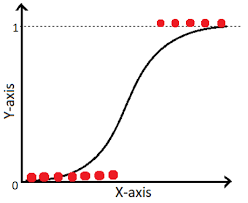
Key Challenges:

1. High Dimensionality: TF-IDF vectorization transforms text into a high-dimensional space (often thousands of dimensions), where each dimension corresponds to a specific word’s frequency or importance in the text. Standard binary logistic regression plots, which typically show decision boundaries in two or three dimensions, cannot naturally extend to this high-dimensional space.

2. Multiclass Classification: Binary logistic regression is inherently designed for two classes. In multiclass settings, logistic regression models typically use schemes like one-vs-rest (OvR) or multinomial logistic regression, which involve multiple binary decisions or probability distributions across more than two classes. This complexity makes it challenging to depict decision boundaries or class separations in a simple 2D or 3D plot.

Alternative Visualization Strategies:

Given these constraints, alternative visualization methods are recommended:

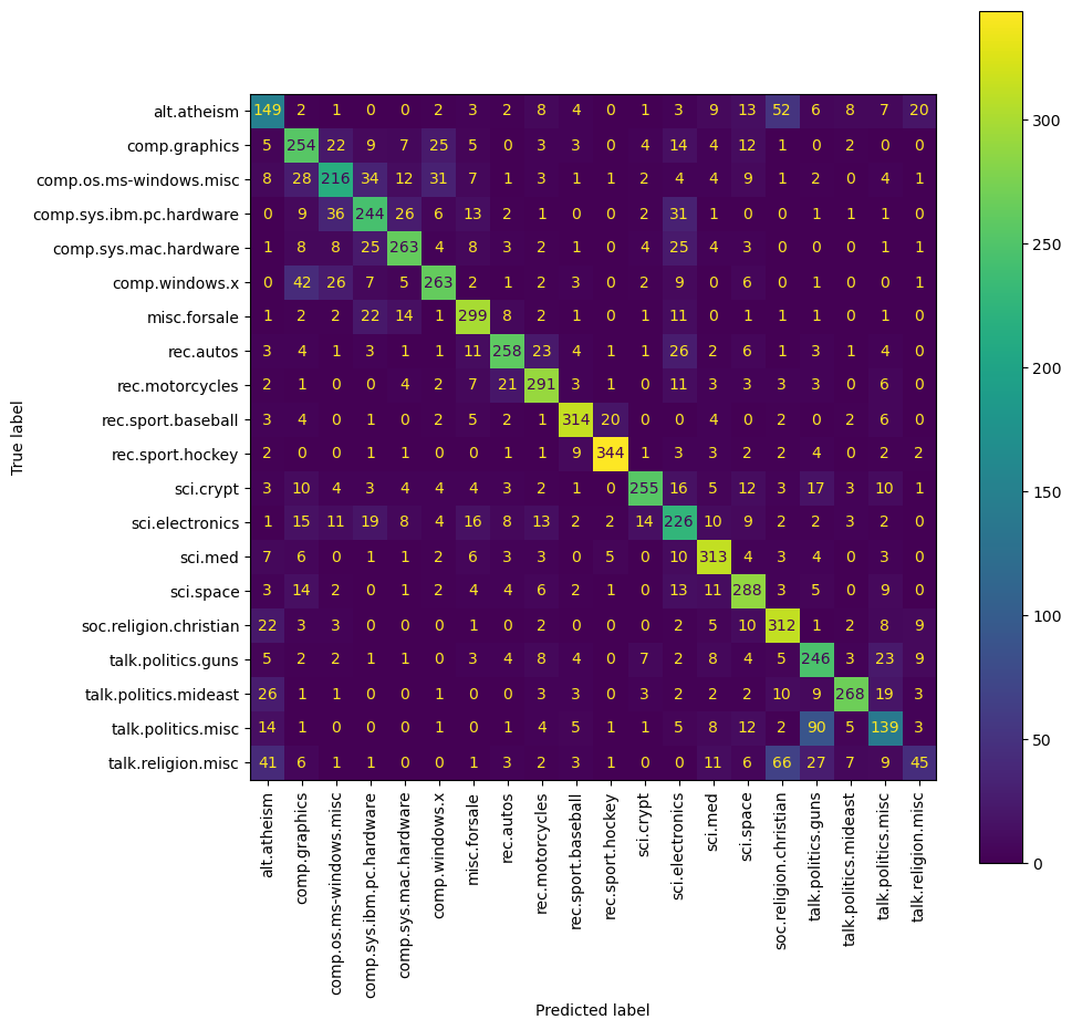
• Confusion Matrix: This is particularly useful in multiclass settings to show the model’s performance across all classes, illustrating how often each class is correctly predicted versus misclassified.

• Dimensionality Reduction: Techniques such as PCA (Principal Component Analysis) or t-SNE (t-Distributed Stochastic Neighbor Embedding) can be used to reduce the dataset to two or three dimensions. These reduced dimensions can then be visualized in a scatter plot, providing a way to observe data clustering and separation at a high level.

These methods provide more meaningful insights into the performance and behavior of logistic regression models in multiclass, high-dimensional scenarios like those involving TF-IDF vectorized text data.

Confusion Matrix

A confusion matrix can help you understand the performance of your classifier across different classes. It shows the actual vs. predicted classifications.

In a confusion matrix for a classification task, the matrix isn’t necessarily symmetrical, meaning the upper and lower sections (above and below the diagonal) aren’t expected to be mirror images of each other. Here’s why:

Understanding the Confusion Matrix

A confusion matrix shows the counts of predictions versus the actual labels:

• Diagonal elements show the number of correct predictions for each class (True Positives for each class).
• Off-diagonal elements show the misclassifications:
  • Elements above the diagonal indicate how many times class X was incorrectly predicted as class Y.
  • Elements below the diagonal indicate how many times class Y was incorrectly predicted as class X.

Reasons for Asymmetry

1. Class Imbalance: If some classes have more samples than others, the likelihood of predicting the majority class increases, affecting the symmetry.

2. Model Biases and Sensitivities: The model might be better at recognizing certain classes over others due to inherent biases in the training data or differences in feature distinctiveness between classes.

3. Error Types:

   • Type I Errors (False Positives): Cases where the model incorrectly predicts the positive class.
   • Type II Errors (False Negatives): Cases where the model fails to predict the positive class when it is the actual class. Each type of error might be more common for certain classes than others.

Example:

Suppose you have three classes: A, B, and C. If:

• Class A is often confused with Class B, but not vice versa.
• Class C is often mistaken for both A and B, but rarely are A or B mistaken for C.

This leads to a non-symmetrical confusion matrix because the misclassification patterns are not uniform across classes.

Interpreting Asymmetries in the Confusion Matrix

A non-symmetrical confusion matrix is typical in practice, especially in multi-class scenarios where varying features, class distributions, and model sensitivities contribute to unique patterns of misclassification. This matrix is a valuable tool for identifying how well the model performs on each class and where it may need improvements or adjustments in its training data or feature selection.

# Compute the confusion matrix
cm = confusion_matrix(y_test, log_pred)
disp = ConfusionMatrixDisplay(confusion_matrix=cm, display_labels=logreg.classes_)

# Plot the confusion matrix
fig, ax = plt.subplots(figsize=(10, 10))
disp.plot(ax=ax, cmap='viridis', xticks_rotation='vertical')  # You can specify the color map
plt.show()

Dimensionality Reduction for Visualization

You can use techniques like PCA (Principal Component Analysis) or t-SNE (t-Distributed Stochastic Neighbor Embedding) to reduce the dimensionality of your TF-IDF vectors to two or three dimensions, and then plot these dimensions.

General PCA Explanation

Principal Components: Each principal component is a linear combination of the original features and represents a direction in the feature space where the data varies the most. Principal components are orthogonal to each other and are ordered by the amount of variance they capture from the data.

• Variance Representation: The first principal component captures the most variance, the second captures the next most, and so on, under the constraint that each is orthogonal to the others.
• Interpretation of Axes: The axes in PCA plots (whether 2D or 3D) represent these principal components. The ticks on these axes indicate the scale or magnitude of the data points along the respective principal components. Since the data often undergoes transformation such as scaling to have zero mean and unit variance before applying PCA, these ticks do not represent the original units of measurement but rather relative positions in the transformed space.

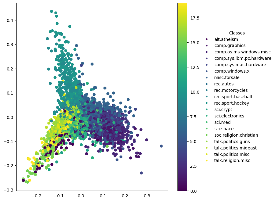
Specific to 2D Plots

In a 2D PCA plot:

• X-axis (First Principal Component): Represents the direction of the greatest variance in the data. This axis captures the largest amount of information (variation) in the dataset.
• Y-axis (Second Principal Component): Represents the direction of the second greatest variance, orthogonal to the first principal component.

Visual Analysis: The plot can reveal clustering and other patterns, helping to visually assess similarities and differences in the data. Points that are close together can be interpreted as having similar characteristics according to the most significant features.

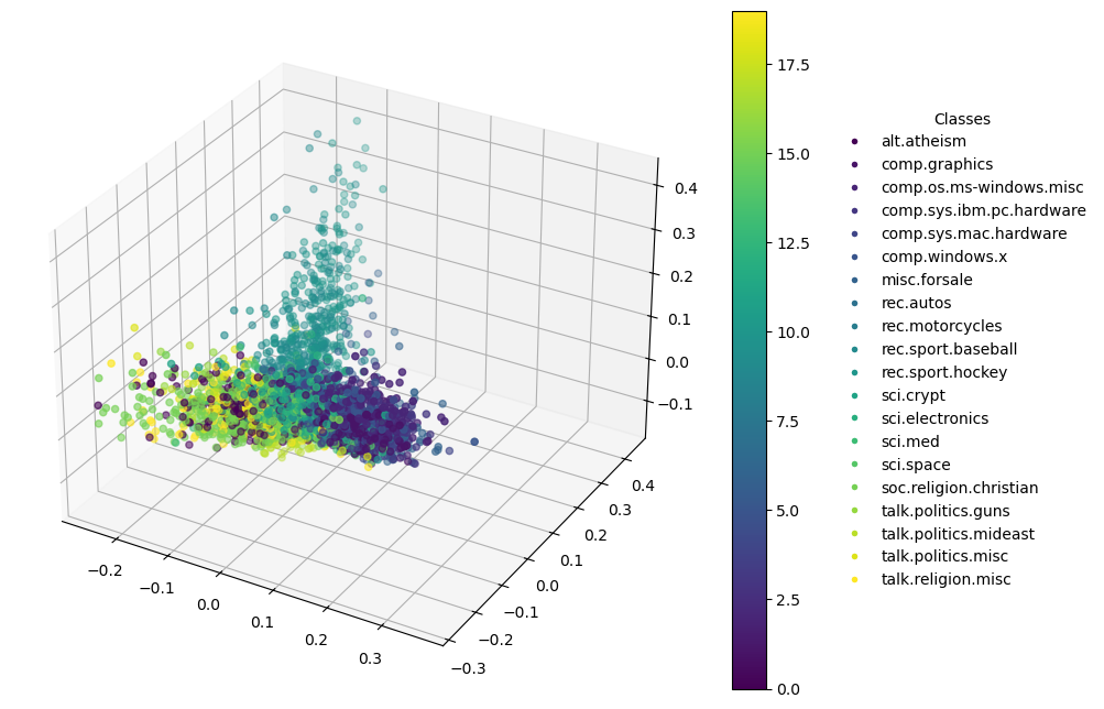
Specific to 3D Plots

In addition to the first and second principal components, 3D PCA plots include:

• Z-axis (Third Principal Component): This axis captures the third highest variance in the data, providing an additional dimension of analysis which is orthogonal to both the first and second components.

Enhanced Visual Analysis: A 3D plot allows for a deeper visual exploration, revealing structures and relationships that might not be visible in 2D. It can be especially useful in datasets where the top two components do not capture the majority of variance.

Practical Use

Both 2D and 3D PCA plots are used for:

• Pattern Recognition: Identifying clusters or outliers in the data.
• Data Simplification: Reducing the dimensionality of the data while attempting to retain the most important characteristics.
• Exploratory Data Analysis: Providing insights into the structure of the data before applying more complex models.

These visualizations serve as powerful tools for initial data analysis, especially when dealing with complex datasets like those generated from text vectorization (e.g., TF-IDF) in natural language processing tasks. They help in making informed decisions about the next steps in the data analysis or machine learning workflow.

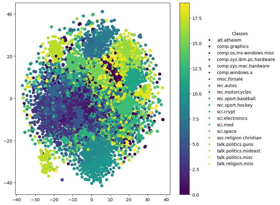
2D Plot

# Reduce dimensions (PCA)
label_encoder = LabelEncoder()
pca = PCA(n_components=2)
X_reduced = pca.fit_transform(x_test.toarray())
y_test_numeric = label_encoder.fit_transform(y_test)

# Plot
plt.figure(figsize=(8, 8))
scatter = plt.scatter(X_reduced[:, 0], X_reduced[:, 1], c=y_test_numeric, cmap='viridis')
plt.colorbar(scatter) 

# Generate legend
classes = label_encoder.classes_
colors = plt.cm.viridis(np.linspace(0, 1, len(classes)))
legend_handles = [Line2D([0], [0], marker='o', color='w', markerfacecolor=col, markersize=5) for col in colors]
plt.legend(legend_handles, classes, title="Classes", bbox_to_anchor=(1.2, 0.5), loc='center left', frameon=False)

# Show the plot
plt.show()

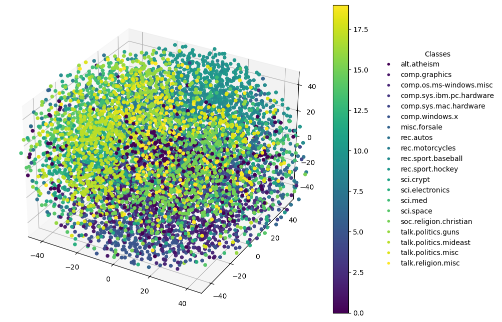
3D Plot

# Fit and transform with PCA for 3 components
label_encoder = LabelEncoder()
pca = PCA(n_components=3)  # Change this to 3 for 3D plotting
X_reduced = pca.fit_transform(x_test.toarray())
y_test_numeric = label_encoder.fit_transform(y_test)

# Create a 3D plot
fig = plt.figure(figsize=(10, 8))
ax = fig.add_subplot(111, projection='3d')  # Add a 3D subplot

# Scatter plot for 3D data
scatter = ax.scatter(X_reduced[:, 0], X_reduced[:, 1], X_reduced[:, 2], c=y_test_numeric, cmap='viridis')

# Color bar
plt.colorbar(scatter, ax=ax)

# Generate legend manually
classes = label_encoder.classes_
colors = plt.cm.viridis(np.linspace(0, 1, len(classes)))
legend_handles = [Line2D([0], [0], marker='o', color='w', markerfacecolor=col, markersize=5) for col in colors]
ax.legend(legend_handles, classes, title="Classes", bbox_to_anchor=(1.2, 0.5), loc='center left', frameon=False)

# Show the plot
plt.show()

General t-SNE Explanation

t-SNE Overview: t-SNE is a non-linear dimensionality reduction technique that is particularly well suited for embedding high-dimensional data into a space of two or three dimensions. The technique is designed to maintain the local structure of the data, making it excellent for visualizing clusters or groups within the data.

• Local Structure Preservation: t-SNE focuses on preserving the local distances between points, meaning that points that are similar in the high-dimensional space are placed near each other in the reduced space. However, global distances (i.e., distances between clusters) might not be as accurately represented.
• Interpretation of Axes: Unlike PCA, t-SNE axes do not have intrinsic meaning as principal components do. The axes in t-SNE plots are abstract and do not correspond to specific original variables. The placement and orientation of clusters can vary significantly between different runs of the algorithm due to its stochastic nature. The axes are simply the 2D or 3D coordinates chosen to best preserve local point-to-point distances.

Specific to 2D Plots

In a 2D t-SNE plot:

• X-axis and Y-axis: These represent the two dimensions onto which the data has been mapped. The axes themselves don’t carry specific meanings but serve as a canvas to observe the grouping and separation of data points.

Visual Analysis: 2D plots are typically sufficient to identify clusters and outliers. They allow for easy visualization of how data points are grouped and which points are similar to each other.

Specific to 3D Plots

A 3D t-SNE plot introduces an additional dimension:

• Z-axis: Adds depth to the visualization, offering another layer for interpreting the data. This can sometimes reveal structures hidden in 2D views.

Enhanced Visual Analysis: 3D plots can provide a more comprehensive view of the data’s structure, revealing relationships that might not be perceptible in only two dimensions. However, they can also be more challenging to interpret and navigate, especially when trying to understand complex data relationships visually.

Practical Use

Both 2D and 3D t-SNE plots are used for:

• Cluster Visualization: Effectively demonstrates how data points are clustered or grouped, which is invaluable for exploratory data analysis, particularly in fields like genomics, image analysis, and text data analysis.
• Outlier Detection: Helps in identifying data points that do not fit well with any group.
• Data Exploration: Provides a means to visually explore the structure of the data, which can guide further analysis or preprocessing steps.

t-SNE is a powerful tool for data visualization, especially when the primary interest is to understand the local structure of the data or to discover patterns in data that lacks clear labels or defined groups.

2D Plot

# Reduce dimensions (t-SNE)
label_encoder = LabelEncoder()
tsne = TSNE(n_components=2, random_state=16)
X_embedded = tsne.fit_transform(x_test.toarray())
y_test_numeric = label_encoder.fit_transform(y_test)

# Plot
plt.figure(figsize=(8, 8))
scatter = plt.scatter(X_embedded[:, 0], X_embedded[:, 1], c=y_test_numeric, cmap='viridis')
plt.colorbar(scatter) 

classes = label_encoder.classes_
colors = plt.cm.viridis(np.linspace(0, 1, len(classes)))
legend_handles = [Line2D([0], [0], marker='o', color='w', markerfacecolor=col, markersize=5) for col in colors]
plt.legend(legend_handles, classes, title="Classes", bbox_to_anchor=(1.2, 0.5), loc='center left', frameon=False)
plt.show()

3D Plot

# Reduce dimensions (t-SNE)
label_encoder = LabelEncoder()
tsne = TSNE(n_components=3, random_state=16)
X_embedded = tsne.fit_transform(x_test.toarray())
y_test_numeric = label_encoder.fit_transform(y_test)

# Create a 3D plot
fig = plt.figure(figsize=(10, 8))
ax = fig.add_subplot(111, projection='3d')  # Add a 3D subplot

# Scatter plot for 3D data
scatter = ax.scatter(X_embedded[:, 0], X_embedded[:, 1], X_embedded[:, 2], c=y_test_numeric, cmap='viridis')

# Adjusting plot limits to exclude outliers
xlims = [np.percentile(X_embedded[:, 0], 5), np.percentile(X_embedded[:, 0], 95)]
ylims = [np.percentile(X_embedded[:, 1], 5), np.percentile(X_embedded[:, 1], 95)]
zlims = [np.percentile(X_embedded[:, 2], 5), np.percentile(X_embedded[:, 2], 95)]

ax.set_xlim(xlims)
ax.set_ylim(ylims)
ax.set_zlim(zlims)

# Color bar
plt.colorbar(scatter, ax=ax)

# Generate legend manually
classes = label_encoder.classes_
colors = plt.cm.viridis(np.linspace(0, 1, len(classes)))
legend_handles = [Line2D([0], [0], marker='o', color='w', markerfacecolor=col, markersize=5) for col in colors]
ax.legend(legend_handles, classes, title="Classes", bbox_to_anchor=(1.2, 0.5), loc='center left', frameon=False)

# Show the plot
plt.show()

Model Coefficients

You can also look at the coefficients of the logistic regression model to determine the importance of each feature (word) but visualizing this effectively can be challenging due to the high number of features. You might want to display the most influential words for each class.

feature_names = np.array(vectorizer.get_feature_names_out())

for class_index in range(logreg.coef_.shape[0]):  # logreg.coef_.shape[0] gives the number of classes
    sorted_coef_index = logreg.coef_[class_index].argsort()
    smallest_coefs = feature_names[sorted_coef_index[:10]]
    largest_coefs = feature_names[sorted_coef_index[:-11:-1]]

    print(f'Class {class_index + 1}')
    print(f'Smallest Coefs:\n{smallest_coefs}\n')
    print(f'Largest Coefs: \n{largest_coefs}\n')

Class 1
Smallest Coefs:
['thanks' 'want' 'email' 'may' 'window' 'work' 'use' 'new' 'game'
 'interested']

Largest Coefs: 
['atheist' 'god' 'religion' 'atheism' 'bobby' 'islam' 'islamic' 'motto'
 'bible' 'argument']

Class 2
Smallest Coefs:
['people' 'list' 'drive' 'right' 'make' 'car' 'key' 'believe' 'god' 'old']

Largest Coefs: 
['graphic' 'image' 'file' 'polygon' 'format' 'program' 'library' 'color'
 'point' 'tiff']

Class 3
Smallest Coefs:
['year' 'would' 'bit' 'car' 'time' 'state' 'course' 'day' 'people' 'game']

Largest Coefs: 
['window' 'file' 'maxaxaxaxaxaxaxaxaxaxaxaxaxaxax' 'driver' 'font'
 'problem' 'do' 'ftpcicaindianaedu' 'win' 'risc']

Class 4
Smallest Coefs:
['people' 'year' 'mac' 'case' 'latest' 'car' 'sun' 'made' 'say' 'life']

Largest Coefs: 
['drive' 'dx' 'card' 'monitor' 'scsi' 'pc' 'controller' 'ide' 'board'
 'disk']

Class 5
Smallest Coefs:
['window' 'do' 'controller' 'pc' 'car' 'group' 'ide' 'god' 'year' 'people']

Largest Coefs: 
['mac' 'apple' 'centris' 'quadra' 'drive' 'lc' 'simms' 'powerbook' 'se'
 'monitor']

Class 6
Smallest Coefs:
['lot' 'go' 'people' 'do' 'driver' 'post' 'card' 'well' 'power' 'said']

Largest Coefs: 
['widget' 'window' 'server' 'motif' 'xr' 'application' 'sun' 'xterm'
 'client' 'display']

Class 7
Smallest Coefs:
['anyone' 'think' 'would' 'could' 'know' 'help' 'might' 'read' 'see'
 'dont']

Largest Coefs: 
['sale' 'offer' 'shipping' 'sell' 'condition' 'new' 'price' 'interested'
 'asking' 'game']

Class 8
Smallest Coefs:
['bike' 'program' 'card' 'file' 'game' 'software' 'book' 'god' 'news'
 'work']

Largest Coefs: 
['car' 'ford' 'engine' 'oil' 'dealer' 'auto' 'toyota' 'wagon'
 'convertible' 'vw']

Class 9
Smallest Coefs:
['program' 'would' 'card' 'could' 'computer' 'believe' 'using' 'software'
 'information' 'please']

Largest Coefs: 
['bike' 'dod' 'motorcycle' 'ride' 'helmet' 'riding' 'rider' 'bmw' 'dog'
 'harley']

Class 10
Smallest Coefs:
['people' 'system' 'car' 'use' 'file' 'problem' 'hockey' 'window' 'would'
 'program']

Largest Coefs: 
['baseball' 'game' 'team' 'player' 'year' 'pitcher' 'cub' 'hit' 'brave'
 'fan']

Class 11
Smallest Coefs:
['use' 'work' 'run' 'system' 'want' 'using' 'drive' 'program' 'file'
 'problem']

Largest Coefs: 
['hockey' 'team' 'game' 'playoff' 'player' 'nhl' 'play' 'season' 'leaf'
 'puck']

Class 12
Smallest Coefs:
['window' 'problem' 'god' 'thanks' 'drive' 'car' 'card' 'help' 'email'
 'please']

Largest Coefs: 
['key' 'clipper' 'encryption' 'nsa' 'chip' 'government' 'security' 'phone'
 'pgp' 'clinton']

Class 13
Smallest Coefs:
['window' 'people' 'think' 'government' 'god' 'mac' 'last' 'posting'
 'year' 'group']

Largest Coefs: 
['circuit' 'electronics' 'voltage' 'chip' 'power' 'line' 'device' 'ground'
 'signal' 'amp']

Class 14
Smallest Coefs:
['god' 'car' 'government' 'drive' 'game' 'someone' 'file' 'system'
 'window' 'card']

Largest Coefs: 
['doctor' 'disease' 'msg' 'patient' 'food' 'treatment' 'medical' 'pain'
 'cancer' 'gordon']

Class 15
Smallest Coefs:
['window' 'car' 'drive' 'game' 'ive' 'card' 'chip' 'computer' 'say' 'best']

Largest Coefs: 
['space' 'orbit' 'nasa' 'launch' 'moon' 'shuttle' 'spacecraft' 'earth'
 'satellite' 'rocket']

Class 16
Smallest Coefs:
['using' 'get' 'system' 'window' 'right' 'car' 'game' 'run' 'file' 'list']

Largest Coefs: 
['god' 'church' 'christian' 'jesus' 'christ' 'christianity' 'sin' 'faith'
 'bible' 'scripture']

Class 17
Smallest Coefs:
['new' 'system' 'god' 'program' 'problem' 'anyone' 'thanks' 'computer'
 'please' 'drive']

Largest Coefs: 
['gun' 'weapon' 'firearm' 'fbi' 'fire' 'jmdcom' 'government' 'law'
 'criminal' 'nra']

Class 18
Smallest Coefs:
['thanks' 'ive' 'im' 'use' 'anyone' 'good' 'email' 'work' 'need' 'please']

Largest Coefs: 
['israel' 'israeli' 'armenian' 'arab' 'jew' 'palestinian' 'turkish'
 'greek' 'turkey' 'turk']

Class 19
Smallest Coefs:
['thanks' 'work' 'window' 'phone' 'chip' 'christian' 'file' 'god' 'game'
 'software']

Largest Coefs: 
['tax' 'homosexual' 'drug' 'government' 'state' 'president' 'clinton'
 'libertarian' 'trial' 'gay']

Class 20
Smallest Coefs:
['anyone' 'thanks' 'need' 'get' 'problem' 'system' 'file' 'use'
 'information' 'window']

Largest Coefs: 
['christian' 'god' 'jesus' 'koresh' 'objective' 'kent' 'bible' 'morality'
 'order' 'rosicrucian']