Introduction to Python for Finance
- Course: DataCamp: Introduction to Python for Finance
- This notebook was created as a reproducible reference.
- The material is from the course
- I completed the exercises
- If you find the content beneficial, consider a DataCamp Subscription.
- Package Versions:
- Pandas version: 2.2.1
- Matplotlib version: 3.8.1
- NumPy version: 1.26.4
My Course Comments
Course Overview: While the course material primarily covers fundamental concepts, making it highly accessible, it has not been included extensively in the Notebook. This approach ensures clarity and focus on practical application rather than overwhelming readers with basic theory.
Recommended Audience: This course is an excellent choice for individuals who are new to Python or those with minimal experience. It provides a solid foundation in Python for financial analysis, equipping beginners with the skills needed to start their journey in data analysis and visualization.
Synopsis
Delve into the world of financial analysis using Python with this beginner-friendly guide. Designed to demonstrate the practical applications of Python through hands-on exercises and real-world examples, this post will equip you with the necessary skills to analyze and visualize financial data effectively.
Key Topics Covered:
Data Manipulation with Pandas: Discover how to leverage Pandas for processing and analyzing financial data. This section will guide you through various techniques that simplify data manipulation, allowing you to make informed decisions based on robust analytics.
Numerical Operations with NumPy: Learn the advantages of using NumPy arrays for numerical operations. This segment explains why arrays are essential for handling large datasets, providing computational efficiency and faster processing capabilities that are crucial in finance.
Data Visualization with Matplotlib: Gain the skills needed to create informative and visually appealing plots. We cover several types of visualizations including line plots, scatter plots, and histograms, showing you how to present financial data in a way that is easy to understand and insightful.
Detailed Insights:
Efficiency with Arrays: Arrays are recommended over lists for large datasets due to their speed and functionality. Using NumPy arrays also ensures uniform data types across the dataset, enhancing the overall performance.
Visualization Techniques: The course introduces practical examples of how to use Matplotlib for data visualization, including an example that plots stock prices over time to illustrate market trends.
Practical Exercises: Through various demonstrations, compare the effectiveness of array operations versus list operations. Also, explore how histograms can be employed to analyze the distribution of P/E ratios within the IT sector, helping identify and discuss outliers.
Real-World Application: A specific case study focuses on the identification and analysis of an outlier in the P/E ratios within the Industrial Technology sector, providing a tangible example of how Python can be used to draw meaningful conclusions from financial data.
Conclusion: This guide serves as an resource for anyone looking to enhance their ability to perform financial analysis using Python. Whether you’re a beginner or looking to sharpen your skills, the techniques and examples provided here will serve as a solid foundation for your journey into financial data analysis.
1
2
3
4
5
6
import pandas as pd
import matplotlib.pyplot as plt
import numpy as np
from numpy import NaN
from glob import glob
import re
1
2
3
pd.set_option('display.max_columns', 200)
pd.set_option('display.max_rows', 300)
pd.set_option('display.expand_frame_repr', True)
Data Files Location
- Most data files for the exercises can be found on the course site
- Other data files may be found in my DataCamp repository
Data File Objects
1
2
3
4
stocks1 = 'data/intro_to_python_for_finance/stock_data.csv'
stocks2 = 'data/intro_to_python_for_finance/stock_data2.csv'
sector_100 = 'data/intro_to_python_for_finance/sector.txt'
exercises = 'data/intro_to_python_for_finance/exercise_data.csv'
Intro to Python for Finance
Course Description
The financial industry is increasingly adopting Python for general-purpose programming and quantitative analysis, ranging from understanding trading dynamics to risk management systems. This course focuses specifically on introducing Python for financial analysis. Using practical examples, you will learn the fundamentals of Python data structures such as lists and arrays and learn powerful ways to store and manipulate financial data to identify trends.
Welcome to Python
This chapter is an introduction to basics in Python, including how to name variables and various data types in Python.
Welcome to Python for Finance!
Comments and Variables
Using variables to evaluate stock trends
$\text{Price to earning ratio} = \frac{\text{Maket Price}}{\text{Earnings per share}}$
1
2
3
4
5
price = 200
earnings = 5

pe_ratio = price/earnings
pe_ratio
1
40.0
Data Types
- integer
- float
- string
- boolean
Check type with:
1
type(variable)
Booleans in Python
Booleans are used to represent True or False statements in Python. Boolean comparisons include:
| Operators | Descriptions |
|---|---|
| > | greater than |
| >= | greater than or equal |
| < | less than |
| <= | less than or equal |
| == | equal (compare) |
| != | does not equal |
Lists
This chapter introduces lists in Python and how they can be used to work with data.
Lists
Nested Lists
List methods and functions
| Methods | Functions |
|---|---|
| All methods are functions | Not all functions are methods |
| List methods are a subset of built in functions in Python | |
| Used on an object | Requires an input of an object |
| prices.sort() | type(prices) |
- Functions take objects as inputs or are “passed” an object
- Methods act on objects
Arrays in Python
This chapter introduces packages in Python, specifically the NumPy package and how it can be efficiently used to manipulate arrays.
Arrays
Why use an array for financial analysis?
- Arrays can handle very large datasets efficiently
- Computationally memory efficient
- Faster calculations and analysis than lists
- Diverse functionality (many functions in Python packages)
- All dtypes in a numpy array are the same
- Each element of a python list keeps its dtype
Array operations
1
2
3
4
5
6
# Arrays - element-wise sum

array_A = np.array([1, 2, 3])
array_B = np.array([4, 5, 6])

array_A + array_B
1
array([5, 7, 9])
1
2
3
4
5
6
# Lists - list concatenation

list_A = [1, 2, 3]
list_B = [4, 5, 6]

list_A + list_B
1
[1, 2, 3, 4, 5, 6]
2D arrays and functions
Using arrays for analysis
Visualization in Python
In this chapter, you will be introduced to the Matplotlib package for creating line plots, scatter plots, and histograms.
Visualization in Python
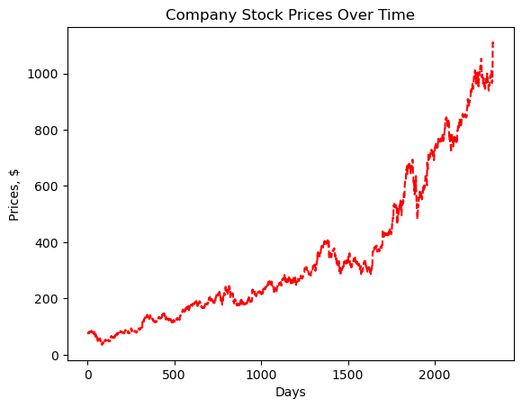
Single Plot
1
2
df = pd.read_csv(stocks1)
df.head()
| Day | Price | |
|---|---|---|
| 0 | 1 | 78.72 |
| 1 | 2 | 78.31 |
| 2 | 3 | 75.98 |
| 3 | 4 | 78.21 |
| 4 | 5 | 78.21 |
1
2
3
4
5
6
7
8
plt.plot(df.Day, df.Price, color='red', linestyle='--')

# Add x and y labels
plt.xlabel('Days')
plt.ylabel('Prices, $')

# Add plot title
plt.title('Company Stock Prices Over Time')
1
Text(0.5, 1.0, 'Company Stock Prices Over Time')
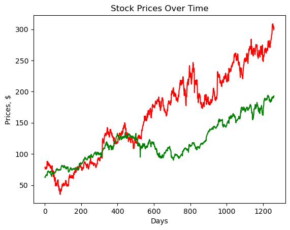
Multiple plots I
1
2
df = pd.read_csv(stocks2)
df.head()
| day | company1 | company2 | |
|---|---|---|---|
| 0 | 1 | 78.72 | 62.957142 |
| 1 | 2 | 78.31 | 62.185715 |
| 2 | 3 | 75.98 | 62.971428 |
| 3 | 4 | 78.21 | 64.279999 |
| 4 | 5 | 78.21 | 64.998573 |
1
2
3
4
5
6
7
8
# Plot two lines of varying colors
plt.plot(df.day, df.company1, color='red')
plt.plot(df.day, df.company2, color='green')

# Add labels
plt.xlabel('Days')
plt.ylabel('Prices, $')
plt.title('Stock Prices Over Time')
1
Text(0.5, 1.0, 'Stock Prices Over Time')
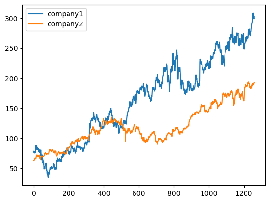
Multiple plots II
1
df[['company1', 'company2']].plot()
1
<Axes: >
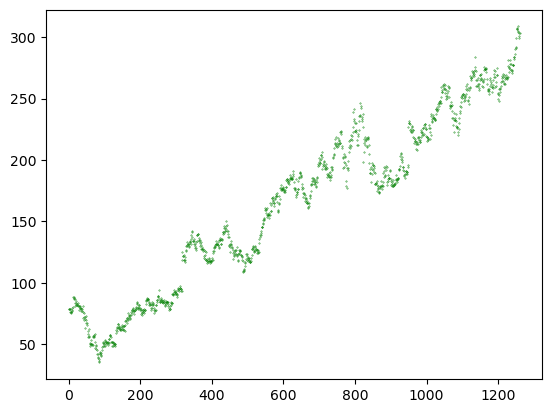
Scatterplots
1
plt.scatter(df.day, df.company1, color='green', s=0.1)
1
<matplotlib.collections.PathCollection at 0x16c390a6c00>
Histograms
- Tell the distribution of the data
- Uses in Finance
- Economic Indicators
- Stock Returns
- Commodity Prices
Why histograms for financial analysis?

- Is you data skewed?
- Is you data centered around the average?
- Do you have any abnormal data points (outliers) in your data?
Histograms and matplotlib.pyplot
1
2
3
import matplotlib.pyplot as plt
plt.hist(x=prices, bins=3)
plt.show()
Normalizing histogram data
1
2
3
import matplotlib.pyplot as plt
plt.hist(x=prices, bins=6, density=True)
plt.show()
- At times it’s beneficial to know the relative frequency or the percentage of observations (rather than frequency counts)
Layering histograms on a plot
1
2
3
plt.hist(x=prices, bins=6, density=True)
plt.hist(x=prices2, bins=6, density=True)
plt.show()
Alpha: Changing transparency of histograms
1
2
3
plt.hist(x=prices, bins=6, density=True, alpha=0.5)
plt.hist(x=prices2, bins=6, density=True, alpha=0.5)
plt.show()
Adding a legend
1
2
3
4
plt.hist(x=prices, bins=6, density=True, alpha=0.5, label='Prices 1')
plt.hist(x=prices2, bins=6, density=True, alpha=0.5, label='Prices New')
plt.legend()
plt.show()
Exercises
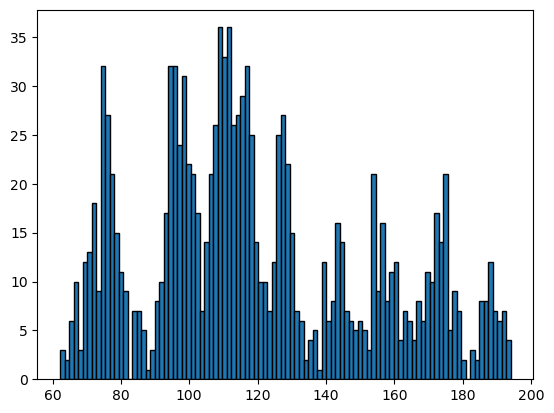
Is data normally distributed?
1
2
plt.hist(df.company2, bins=100, ec='black')
plt.show()
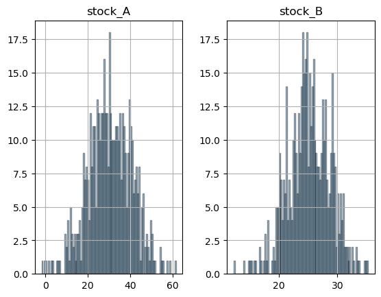
Comparing two histograms
1
2
df_exercises = pd.read_csv(exercises)
df_exercises.head()
| stock_A | stock_B | |
|---|---|---|
| 0 | 45.057678 | 19.993790 |
| 1 | 45.687739 | 31.135599 |
| 2 | 10.257555 | 25.024954 |
| 3 | 27.169681 | 22.220461 |
| 4 | 32.796236 | 21.218579 |
pd.DataFrame.hist
1
2
df_exercises.hist(bins=100, alpha=0.4, ec='black')
plt.show()
matplotlib.pyplt as plt
1
2
3
4
5
6
7
8
9
10
11
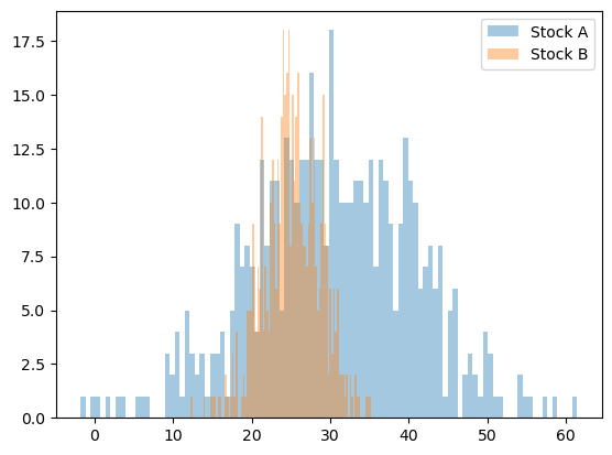
# Plot histogram of stocks_A
plt.hist(df_exercises.stock_A, bins=100, alpha=0.4, label='Stock A')
# Plot histogram of stocks_B
plt.hist(df_exercises.stock_B, bins=100, alpha=0.4, label='Stock B')
# Add the legend
plt.legend()
# Display plot
plt.show()
S&P 100 Case Study
In this chapter, you will get a chance to apply all the techniques you learned in the course on the S&P 100 data.
Introducing the dataset
Overall Review
- Python shell and scripts
- Variables and data types
- Lists
- Arrays
- Methods and functions
- Indexing and subsetting
- Matplotlib
S&P 100 Companies
Standard and Poor’s S&P 100:
- made up of major companies that span multiple industry groups
- used to measure stock performance of large companies
S&P 100 Sectors

The Data
- EPS: earning per share
1
2
df = pd.read_csv(sector_100)
df.head()
| Name | Sector | Price | EPS | |
|---|---|---|---|---|
| 0 | Apple Inc | Information Technology | 170.12 | 9.20 |
| 1 | Abbvie Inc | Health Care | 93.29 | 5.31 |
| 2 | Abbott Laboratories | Health Care | 55.28 | 2.41 |
| 3 | Accenture Plc | Information Technology | 145.30 | 5.91 |
| 4 | Allergan Plc | Health Care | 171.81 | 15.42 |
1
df.tail()
| Name | Sector | Price | EPS | |
|---|---|---|---|---|
| 97 | Verizon Communications Inc | Telecommunications | 45.85 | 3.75 |
| 98 | Walgreens Boots Alliance | Consumer Staples | 70.25 | 5.10 |
| 99 | Wells Fargo & Company | Financials | 54.02 | 4.14 |
| 100 | Wal-Mart Stores | Consumer Staples | 96.08 | 4.36 |
| 101 | Exxon Mobil Corp | Energy | 80.31 | 3.56 |
Price to Earnings Ratio
$\text{Price to earning ratio} = \frac{\text{Maket Price}}{\text{Earnings per share}}$
- The dollar amount one can expect to invest in a company in order to receive one dollar of the company’s earnings
- The ratio for valuing a company that measures its current share price relative to the per-share earnings
- In general, higher P/E ratio idicates higher growth expectations
Case Study Objective I:
Given
- List of data describing the S&P 100: names, prices, earnigns, sectors
Objective Part I
- Explore and analyze the S&P 100 data, specifically the P/E ratios of S&P 100 companies
Methods
- Step 1: examine the lists
- Step 2: Convert lists to arrays
- Step 3: Elementwise array operations
Project Explorations
Data
1
2
3
4
names = df.Name.values
prices = df.Price.values
earnings = df.EPS.values
sectors = df.Sector.values
1
type(names)
1
numpy.ndarray
Lists
Stocks in the S&P 100 are selected to represent sector balance and market capitalization. To begin, let’s take a look at what data we have associated with S&P companies.
Four lists, names, prices, earnings, and sectors, are available in your workspace.
Instructions
- Print the first four items in names.
- Print the name, price, earning, and sector associated with the last company in the lists.
1
2
3
4
5
6
7
8
# First four items of names
print(names[:4])

# Print information on last company
print(names[-1])
print(prices[-1])
print(earnings[-1])
print(sectors[-1])
1
2
3
4
5
['Apple Inc' 'Abbvie Inc' 'Abbott Laboratories' 'Accenture Plc']
Exxon Mobil Corp
80.31
3.56
Energy
Arrays and NumPy
NumPy is a scientific computing package in Python that helps you to work with arrays. Let’s use array operations to calculate price to earning ratios of the S&P 100 stocks.
The S&P 100 data is available as the lists: prices (stock prices per share) and earnings (earnings per share).
Instructions
- Import the numpy as np.
- Convert the prices and earnings lists to arrays, prices_array and earnings_array, respectively.
- Calculate the price to earnings ratio as pe.
1
2
3
# Convert lists to arrays
prices_array = np.array(prices)
earnings_array = np.array(earnings)
1
2
3
# Calculate P/E ratio
pe = prices/earnings
pe[:10]
1
2
3
array([ 18.49130435,  17.56873823,  22.93775934,  24.58544839,
        11.14202335,  23.70517928,  14.8011782 ,  13.42845787,
       285.99492386,  17.99233716])
A closer look at sectors
Case Study Objective II:
Given
- Numpy arrays of data describing the S&P 100: names, prices, earnings, sectors
Objective Part II
- Explore and analyze sector-specific P/E ratios within companies of the S&P 100
Methods
- Step 1: Create a boolean filtering array
- Step 2: Apply filtering array to subset another array
- Step 3: Summarize P/E ratios
- Calculate the average and standard deviation of these sector-specific P/E ratios
Project Explorations
Filtering arrays
In this lesson, you will focus on two sectors:
- Information Technology
- Consumer Staples
numpy is imported as np and S&P 100 data is stored as arrays: names, sectors, and pe (price to earnings ratio).
Instructions 1/2
- Create a boolean array to determine which elements in sectors are ‘Information Technology’.
- Use the boolean array to subset names and pe in the Information Technology sector.
1
2
3
4
5
6
7
8
9
10
# Create boolean array
boolean_array = (sectors == 'Information Technology')

# Subset sector-specific data
it_names = names[boolean_array]
it_pe = pe[boolean_array]

# Display sector names
print(it_names)
print(it_pe)
1
2
3
4
5
6
7
['Apple Inc' 'Accenture Plc' 'Cisco Systems Inc' 'Facebook Inc'
 'Alphabet Class C' 'Alphabet Class A' 'International Business Machines'
 'Intel Corp' 'Mastercard Inc' 'Microsoft Corp' 'Oracle Corp'
 'Paypal Holdings' 'Qualcomm Inc' 'Texas Instruments' 'Visa Inc']
[18.49130435 24.58544839 16.76497696 34.51637765 34.09708738 34.6196853
 11.08345534 14.11320755 34.78654292 24.40532544 19.20392157 54.67857143
 17.67989418 24.28325123 31.68678161]
Instructions 2/2
- Create a boolean array to determine which elements in sectors are ‘Consumer Staples’.
- Use the boolean array to subset names and pe in the Consumer Staples sector.
1
2
3
4
5
6
7
8
9
10
# Create boolean array
boolean_array = (sectors == 'Consumer Staples')

# Subset sector-specific data
cs_names = names[boolean_array]
cs_pe = pe[boolean_array]

# Display sector names
print(cs_names)
print(cs_pe)
1
2
3
4
5
6
7
['Colgate-Palmolive Company' 'Costco Wholesale' 'CVS Corp'
 'Kraft Heinz Co' 'Coca-Cola Company' 'Mondelez Intl Cmn A' 'Altria Group'
 'Pepsico Inc' 'Procter & Gamble Company'
 'Philip Morris International Inc' 'Walgreens Boots Alliance'
 'Wal-Mart Stores']
[25.14285714 29.41924399 12.29071804 22.63764045 24.12698413 20.72682927
 21.04746835 22.55859375 22.19346734 23.01781737 13.7745098  22.03669725]
Summarizing sector data
In this exercise, you will calculate the mean and standard deviation of P/E ratios for Information Technology and Consumer Staples sectors. numpy is imported as np and the it_pe and cs_pe arrays from the previous exercise are available in your workspace.
Instructions 1/2
Calculate the mean and standard deviation of the P/E ratios (it_pe) for the Industrial Technology sector.
1
2
3
4
5
6
# Calculate mean and standard deviation
it_pe_mean = np.mean(it_pe)
it_pe_std = np.std(it_pe)

print(it_pe_mean)
print(it_pe_std)
1
2
26.333055420408595
10.8661467926753
Instructions 2/2
- Calculate the mean and standard deviation of the P/E ratios (cs_pe) for the Consumer Staples sector.
1
2
3
4
5
6
# Calculate mean and standard deviation
cs_pe_mean = np.mean(cs_pe)
cs_pe_std = np.std(cs_pe)

print(cs_pe_mean)
print(cs_pe_std)
1
2
21.581068906419564
4.412021654267338
Plot P/E ratios
Let’s take a closer look at the P/E ratios using a scatter plot for each company in these two sectors.
The arrays it_pe and cs_pe from the previous exercise are available in your workspace. Also, each company name has been assigned a numeric ID contained in the arrays it_id and cs_id.
Instructions
- Draw a scatter plot of it_pe ratios with red markers and ‘IT’ label.
- On the same plot, add the cs_pe ratios with green markers and ‘CS’ label.
- Add a legend to this plot.
- Display the plot.
1
2
3
4
5
6
7
8
9
10
11
12
13
14
it_id = np.arange(0, 15)
cs_id = np.arange(0, 12)

# Make a scatterplot
plt.scatter(it_id, it_pe, color='red', label='IT')
plt.scatter(cs_id, cs_pe, color='green', label='CS')

# Add legend
plt.legend()

# Add labels
plt.xlabel('Company ID')
plt.ylabel('P/E Ratio')
plt.show()
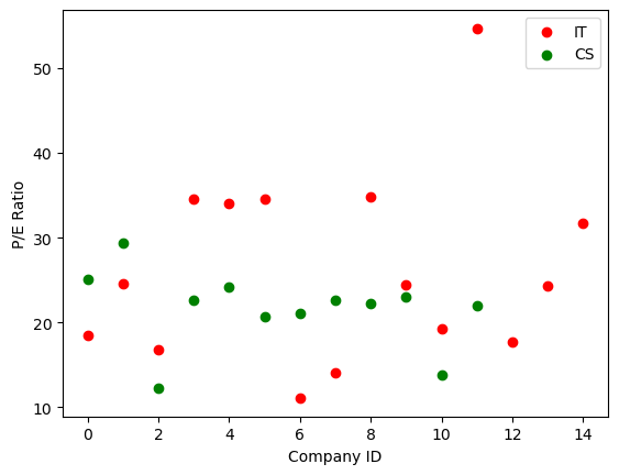
Notice that there is one company in the IT sector with an unusually high P/E ratio
Visualizating trends
Case Study Objective III:
Objective Part III
- Investigate the outlier from the scatter plot
Methods
- Step 1: Make a histogram of the P/E ratios
- Step 2:
- Identify the outlier P/E ratio
- Create a boolean array filter to subset this company
- Filter out this company information from the provided datasets
Project Explorations
Histogram of P/E ratios
To visualize and understand the distribution of the P/E ratios in the IT sector, you can use a histogram.
The array it_pe from the previous exercise is available in your workspace.
Instructions
- Selectively import the pyplot module of matplotlib as plt.
- Plot a histogram of it_pe with 8 bins.
- Add the x-label as ‘P/E ratio’ and y-label as ‘Frequency’.
- Display the plot.
1
2
3
4
5
6
7
8
9
10
11
# Plot histogram
plt.hist(it_pe, bins=8, ec='black')

# Add x-label
plt.xlabel('P/E ratio')

# Add y-label
plt.ylabel('Frequency')

# Show plot
plt.show()
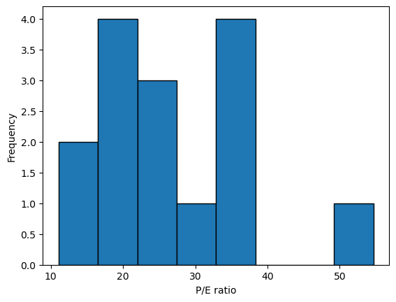
Identify the outlier
- Histograms can help you to identify outliers or abnormal data points. Which P/E ratio in this histogram is an example of an outlier?
A stock with P/E ratio > 50.
Name the outlier
You’ve identified that a company in the Industrial Technology sector has a P/E ratio of greater than 50. Let’s identify this company.
numpy is imported as np, and arrays it_pe (P/E ratios of Industrial Technology companies) and it_names (names of Industrial Technology companies) are available in your workspace.
Instructions
- Identify the P/E ratio greater than 50 and assign it to outlier_price.
- Identify the company with P/E ratio greater than 50 and assign it to outlier_name.
1
2
3
4
5
6
7
8
# Identify P/E ratio within it_pe that is > 50
outlier_price = it_pe[it_pe > 50]

# Identify the company with PE ratio > 50
outlier_name = it_names[it_pe == outlier_price]

# Display results
print(f'In 2017 {outlier_name[0]} had an abnormally high P/E ratio of {round(outlier_price[0], 2)}.')
1
In 2017 Paypal Holdings had an abnormally high P/E ratio of 54.68.
Certificate